Section 3.2 The Second Way to Compute Determinant

Observation 3.2.1. Compute the determinant.

Consider an upper triangular matrix of the form:
\begin{equation*} \begin{bmatrix} a_{11} \amp a_{12} \amp a_{13} \amp \cdots \amp a_{1,n-1} \amp a_{1n}\\ 0 \amp a_{22} \amp a_{23} \amp \cdots \amp a_{2,n-1} \amp a_{2n}\\ 0 \amp 0 \amp a_{33} \amp \cdots \amp a_{3,n-1} \amp a_{3n}\\ \vdots \amp \vdots \amp \vdots \amp \ddots \amp \vdots \amp \vdots\\ 0 \amp 0 \amp 0 \amp \cdots \amp a_{n-1,n-1} \amp a_{n-1,n}\\ 0 \amp 0 \amp 0 \amp \cdots \amp 0 \amp a_{nn} \end{bmatrix} \end{equation*}
Questions to consider:
  1. What is the determinant of this matrix?
  2. Is there way to turn a matrix into this form?
In this section, we will explore how to compute determinants efficiently and understand their fundamental properties.

Subsection 3.2.1 Fast way to get the determinant

You may use A.det() to get the determinant of matrix A in SageMath.

Activity 3.2.1.

Find the determinant of the matrix
\begin{equation*} A = \left[\begin{array}{rrrr} 2 \amp 1 \amp -2 \amp -3 \\ 3 \amp 0 \amp -1 \amp -2 \\ -3 \amp 4 \amp 1 \amp 2\\ 1 \amp 3 \amp 3 \amp -1 \\ \end{array}\right]\text{.} \end{equation*}

Activity 3.2.2. Exercise.

Find the determinant of the matrix
\begin{equation*} B = \left[\begin{array}{rrr} 1 \amp 2 \amp 3\\ 0 \amp 1 \amp 4\\ 5 \amp 6 \amp 0 \end{array}\right]\text{.} \end{equation*}

Subsection 3.2.2 Elementary Row Operations and Determinants

In the previous activities, we learned how to compute determinants using cofactor expansion. However, for large matrices, this method can be computationally intensive. In this subsection, we explore how elementary row operations affect determinants, which will lead to more efficient computational methods.

Activity 3.2.3. Exploring Effects of Row Operations on Determinants.

Recall the matrix \(A\) from Activity 3.2.1:
\begin{equation*} A = \left[\begin{array}{rrrr} 2 \amp 1 \amp -2 \amp -3 \\ 3 \amp 0 \amp -1 \amp -2 \\ -3 \amp 4 \amp 1 \amp 2\\ 1 \amp 3 \amp 3 \amp -1 \\ \end{array}\right] \end{equation*}
In next activity, we perform three elementary row operations to yield matrices, and then find the determinants, respectively.
Swap the rows 2 and 3 to yield the matrix
\begin{equation*} B = \left[\begin{array}{rrrr} 2 \amp 1 \amp -2 \amp -3 \\ -3 \amp 4 \amp 1 \amp 2\\ 3 \amp 0 \amp -1 \amp -2 \\ 1 \amp 3 \amp 3 \amp -1 \\ \end{array}\right]\text{.} \end{equation*}
Find the determinant of \(B\text{,}\) and state what you find.
\(C = \left[\begin{array}{rrrr} 2 \amp 1 \amp -2 \amp -3 \\ 9 \amp 0 \amp -3 \amp -6 \\ -3 \amp 4 \amp 1 \amp 2\\ 1 \amp 3 \amp 3 \amp -1 \\ \end{array}\right]\) is obtained by scaling row 2 of the matrix \(A\) by 3. Find the determinant of \(C\text{,}\) and state what you find.
Let \(D = \left[\begin{array}{rrrr} 2 \amp 1 \amp -2 \amp -3 \\ 3 \amp 0 \amp -1 \amp -2 \\ -3 \amp 4 \amp 1 \amp 2\\ 7 \amp 3 \amp 1 \amp -5 \\ \end{array}\right]\) be obtained by adding 2 times row 2 of the matrix \(A\) to row 4. Find the determinant of \(D\text{,}\) and state what you find.
Based on your computations, what patterns do you observe? How does each type of row operation affect the determinant?
The patterns observed in the activity above are not coincidental. They reflect fundamental properties of determinants that we now state formally.

Proof.

We prove each part separately.
Part 1: Multiplying a row by a scalar
Suppose \(B\) is obtained from \(A\) by multiplying row \(i\) by scalar \(k\text{.}\) Using cofactor expansion along row \(i\text{:}\)
\begin{align*} \det(B) \amp= \sum_{j=1}^{n} b_{ij}C_{ij}\\ \amp= \sum_{j=1}^{n} (ka_{ij})C_{ij}\\ \amp= k\sum_{j=1}^{n} a_{ij}C_{ij}\\ \amp= k\det(A) \end{align*}
Note that the cofactors \(C_{ij}\) are the same for both \(A\) and \(B\text{,}\) since they depend on minors that do not involve row \(i\text{.}\)
Part 2: Row replacement
Suppose \(B\) is obtained from \(A\) by adding \(c\) times row \(j\) to row \(i\) (where \(i \neq j\)). Let’s denote the rows of \(A\) as \(\mathbf{r}_1, \mathbf{r}_2, \ldots, \mathbf{r}_n\text{.}\) Then \(B\) has row \(i\) equal to \(\mathbf{r}_i + c\mathbf{r}_j\text{,}\) while all other rows remain unchanged.
Using the linearity property of determinants in a single row (which follows from cofactor expansion):
\begin{equation*} \det(B) = \det[\mathbf{r}_1, \ldots, \mathbf{r}_i + c\mathbf{r}_j, \ldots, \mathbf{r}_n] \end{equation*}
\begin{equation*} = \det[\mathbf{r}_1, \ldots, \mathbf{r}_i, \ldots, \mathbf{r}_n] + c\det[\mathbf{r}_1, \ldots, \mathbf{r}_j, \ldots, \mathbf{r}_n] \end{equation*}
The first determinant is \(\det(A)\text{.}\) The second determinant has two identical rows (row \(i\) and row \(j\) are both \(\mathbf{r}_j\)), so it equals zero. Therefore, \(\det(B) = \det(A)\text{.}\)
Part 3: Row interchange
We first prove a lemma: if \(A\) has two identical rows, then \(\det(A) = 0\text{.}\)
Proof of lemma: Suppose rows \(i\) and \(j\) of \(A\) are identical (with \(i \lt j\)). If we interchange these two rows to obtain matrix \(B\text{,}\) then \(B = A\text{.}\) However, by the row interchange property we’re trying to prove, we would have \(\det(B) = -\det(A)\text{.}\) Since \(B = A\text{,}\) we have \(\det(A) = -\det(A)\text{,}\) which implies \(2\det(A) = 0\text{,}\) so \(\det(A) = 0\text{.}\)
Now we prove Part 3. Let \(B\) be obtained from \(A\) by interchanging rows \(i\) and \(j\) (with \(i \lt j\)). Consider the matrix \(C\) obtained from \(A\) by:
  • Adding row \(j\) to row \(i\) (so row \(i\) of \(C\) equals \(\mathbf{r}_i + \mathbf{r}_j\))
By Part 2, \(\det(C) = \det(A)\text{.}\) Now perform these operations on \(C\text{:}\)
  • Subtract row \(i\) from row \(j\text{:}\) row \(j\) becomes \(\mathbf{r}_j - (\mathbf{r}_i + \mathbf{r}_j) = -\mathbf{r}_i\)
  • Multiply row \(j\) by \(-1\text{:}\) row \(j\) becomes \(\mathbf{r}_i\)
  • Subtract row \(j\) from row \(i\text{:}\) row \(i\) becomes \((\mathbf{r}_i + \mathbf{r}_j) - \mathbf{r}_i = \mathbf{r}_j\)
After these operations, we obtain matrix \(B\text{.}\) By Parts 1 and 2:
\begin{equation*} \det(B) = (-1)\det(C) = -\det(A) \end{equation*}
Alternatively, a more direct proof uses mathematical induction on \(n\text{,}\) the size of the matrix, combined with cofactor expansion.
This theorem has a profound interpretation in terms of elementary matrices.

Proof.

Recall that an elementary matrix \(E\) is obtained by performing a single elementary row operation on the identity matrix \(I\text{.}\) The matrix \(EA\) is the result of performing the same elementary row operation on \(A\text{.}\)
We consider three cases corresponding to the three types of elementary row operations:
Case 1: \(E\) is obtained by multiplying one row of \(I\) by \(k \neq 0\text{.}\) Then \(\det(E) = k\) (since the determinant of a diagonal matrix is the product of its diagonal entries, and \(E\) has one diagonal entry equal to \(k\) and all others equal to \(1\)).
By Theorem 3.2.2 Part 1, \(\det(EA) = k\det(A) = \det(E)\det(A)\text{.}\)
Case 2: \(E\) is obtained by adding a multiple of one row to another row of \(I\text{.}\) In this case, \(\det(E) = \det(I) = 1\text{.}\)
By Theorem 3.2.2 Part 2, \(\det(EA) = \det(A) = 1 \cdot \det(A) = \det(E)\det(A)\text{.}\)
Case 3: \(E\) is obtained by interchanging two rows of \(I\text{.}\) Then \(\det(E) = -\det(I) = -1\text{.}\)
By Theorem 3.2.2 Part 3, \(\det(EA) = -\det(A) = \det(E)\det(A)\text{.}\)
In all cases, we have \(\det(EA) = \det(E)\det(A)\text{.}\)

Proof.

Let \(E\) be the elementary matrix obtained by multiplying one row of the identity matrix \(I_n\) by \(k\text{.}\) Then \(\det(E) = k\text{.}\)
Notice that \(kA\) can be obtained by multiplying each of the \(n\) rows of \(A\) by \(k\text{.}\) This is equivalent to multiplying \(A\) by \(n\) elementary matrices of the form \(E\text{,}\) one for each row.
More formally, if \(E_1, E_2, \ldots, E_n\) are elementary matrices where \(E_i\) multiplies row \(i\) by \(k\text{,}\) then \(kA = E_n E_{n-1} \cdots E_1 A\text{.}\)
By repeated application of Proposition 3.2.3:
\begin{align*} \det(kA) \amp= \det(E_n E_{n-1} \cdots E_1 A)\\ \amp= \det(E_n)\det(E_{n-1})\cdots\det(E_1)\det(A)\\ \amp= k \cdot k \cdots k \cdot \det(A) \quad \text{( factors of )}\\ \amp= k^n \det(A) \end{align*}

Insight 3.2.6. Computational Strategy.

Theorem 3.2.2 provides an efficient method for computing determinants:
  1. Use elementary row operations to reduce the matrix to an echelon form (typically upper triangular).
  2. Keep track of how each operation affects the determinant (multiply by \(k\text{,}\) multiply by \(-1\text{,}\) or leave unchanged).
  3. For an upper triangular matrix, the determinant is simply the product of the diagonal entries.
Key observation: It is more efficient to compute the determinant of a matrix through its echelon form rather than using cofactor expansion, especially for large matrices.

Example 3.2.7. Computing Determinant Using Row Operations.

Compute \(\det(A)\) where
\begin{equation*} A = \left[\begin{array}{rrr} 1 \amp -4 \amp 2 \\ -2 \amp 8 \amp -9 \\ -1 \amp 7 \amp 0 \end{array}\right] \end{equation*}
Solution.
We reduce \(A\) to echelon form using row operations:
\begin{align*} A \amp= \left[\begin{array}{rrr} 1 \amp -4 \amp 2 \\ -2 \amp 8 \amp -9 \\ -1 \amp 7 \amp 0 \end{array}\right]\\ \xrightarrow{R_2 + 2R_1} \amp \left[\begin{array}{rrr} 1 \amp -4 \amp 2 \\ 0 \amp 0 \amp -5 \\ -1 \amp 7 \amp 0 \end{array}\right] \quad (\det \text{ unchanged})\\ \xrightarrow{R_3 + R_1} \amp \left[\begin{array}{rrr} 1 \amp -4 \amp 2 \\ 0 \amp 0 \amp -5 \\ 0 \amp 3 \amp 2 \end{array}\right] \quad (\det \text{ unchanged})\\ \xrightarrow{R_2 \leftrightarrow R_3} \amp \left[\begin{array}{rrr} 1 \amp -4 \amp 2 \\ 0 \amp 3 \amp 2 \\ 0 \amp 0 \amp -5 \end{array}\right] \quad (\det \text{ changes sign}) \end{align*}
The final matrix is upper triangular with determinant \(1 \cdot 3 \cdot (-5) = -15\text{.}\)
Since we performed one row interchange, we have:
\begin{equation*} \det(A) = -(-15) = 15 \end{equation*}

Proof.

(\(\Rightarrow\)) Suppose \(A\) is invertible. Then \(A\) is row equivalent to the identity matrix \(I\text{.}\) This means there exist elementary matrices \(E_1, E_2, \ldots, E_m\) such that
\begin{equation*} E_m E_{m-1} \cdots E_1 A = I \end{equation*}
Taking determinants of both sides and using Proposition 3.2.3:
\begin{equation*} \det(E_m)\det(E_{m-1})\cdots\det(E_1)\det(A) = \det(I) = 1 \end{equation*}
Since each elementary matrix has a non-zero determinant (either \(k \neq 0\text{,}\) \(1\text{,}\) or \(-1\)), we conclude that \(\det(A) \neq 0\text{.}\)
(\(\Leftarrow\)) Suppose \(\det(A) \neq 0\text{.}\) We prove by contradiction that \(A\) is invertible.
Suppose \(A\) is not invertible. Then \(A\) is not row equivalent to \(I\text{,}\) which means when we reduce \(A\) to row echelon form, we obtain at least one zero row. Let \(U\) be the row echelon form of \(A\text{.}\) Then there exist elementary matrices \(E_1, \ldots, E_m\) such that
\begin{equation*} U = E_m E_{m-1} \cdots E_1 A \end{equation*}
Since \(U\) has a zero row, \(\det(U) = 0\) (by cofactor expansion along the zero row). By Proposition 3.2.3:
\begin{equation*} 0 = \det(U) = \det(E_m)\det(E_{m-1})\cdots\det(E_1)\det(A) \end{equation*}
Since each \(\det(E_i) \neq 0\text{,}\) we must have \(\det(A) = 0\text{,}\) which contradicts our assumption. Therefore, \(A\) must be invertible.

Proof.

We consider two cases.
Case 1: Suppose \(A\) is not invertible. Then \(\det(A) = 0\) by Theorem 3.2.8. We need to show that \(\det(AB) = 0\text{.}\)
Since \(A\) is not invertible, the columns of \(A\) are linearly dependent. This means there exists a non-zero vector \(\mathbf{x}\) such that \(A\mathbf{x} = \mathbf{0}\text{.}\)
The columns of \(AB\) are \(AB\mathbf{e}_1, AB\mathbf{e}_2, \ldots, AB\mathbf{e}_n\text{,}\) where \(\mathbf{e}_i\) are the standard basis vectors. If \(B\mathbf{x} = c_1\mathbf{e}_1 + c_2\mathbf{e}_2 + \cdots + c_n\mathbf{e}_n\) for some scalars \(c_i\text{,}\) then:
\begin{align*} AB\mathbf{x} \amp= A(B\mathbf{x})\\ \amp= A(c_1\mathbf{e}_1 + \cdots + c_n\mathbf{e}_n)\\ \amp= c_1(AB\mathbf{e}_1) + \cdots + c_n(AB\mathbf{e}_n)\\ \amp= \mathbf{0} \end{align*}
If \(B\mathbf{x} \neq \mathbf{0}\text{,}\) then the columns of \(AB\) are linearly dependent, so \(AB\) is not invertible, and thus \(\det(AB) = 0\text{.}\)
If \(B\mathbf{x} = \mathbf{0}\) for all \(\mathbf{x}\) with \(A\mathbf{x} = \mathbf{0}\text{,}\) then the null space of \(A\) is contained in the null space of \(B\text{,}\) which again implies that \(AB\) is not invertible.
Therefore, in this case, \(\det(AB) = 0 = \det(A)\det(B)\text{.}\)
Case 2: Suppose \(A\) is invertible. Then \(A\) can be written as a product of elementary matrices:
\begin{equation*} A = E_1 E_2 \cdots E_m \end{equation*}
Then:
\begin{align*} \det(AB) \amp= \det(E_1 E_2 \cdots E_m B)\\ \amp= \det(E_1)\det(E_2 \cdots E_m B) \quad \text{(by \knowl{./knowl/xref/prop-elementary-matrix-det.html}{\text{Proposition 3.2.3}})}\\ \amp= \det(E_1)\det(E_2)\det(E_3 \cdots E_m B)\\ \amp\vdots\\ \amp= \det(E_1)\det(E_2)\cdots\det(E_m)\det(B)\\ \amp= \det(E_1 E_2 \cdots E_m)\det(B)\\ \amp= \det(A)\det(B) \end{align*}
Therefore, in both cases, \(\det(AB) = \det(A)\det(B)\text{.}\)

Proof.

Since \(AA^{-1} = I\text{,}\) we have:
\begin{equation*} \det(AA^{-1}) = \det(I) = 1 \end{equation*}
\begin{equation*} \det(A)\det(A^{-1}) = 1 \end{equation*}
Therefore, \(\det(A^{-1}) = \dfrac{1}{\det(A)}\text{.}\)

Example 3.2.11. Applying the Determinant Product Theorem.

Let \(A = \begin{bmatrix} 1 \amp 2 \\ 3 \amp 4 \end{bmatrix}\) and \(B = \begin{bmatrix} 2 \amp 0 \\ 1 \amp 3 \end{bmatrix}\text{.}\)
Verify that \(\det(AB) = \det(A)\det(B)\text{.}\)
Solution.
First, compute the individual determinants:
\begin{align*} \det(A) \amp= 1(4) - 2(3) = 4 - 6 = -2\\ \det(B) \amp= 2(3) - 0(1) = 6\\ \det(A)\det(B) \amp= (-2)(6) = -12 \end{align*}
Now compute \(AB\) and its determinant:
\begin{align*} AB \amp= \begin{bmatrix} 1 \amp 2 \\ 3 \amp 4 \end{bmatrix}\begin{bmatrix} 2 \amp 0 \\ 1 \amp 3 \end{bmatrix}\\ \amp= \begin{bmatrix} 1(2)+2(1) \amp 1(0)+2(3) \\ 3(2)+4(1) \amp 3(0)+4(3) \end{bmatrix}\\ \amp= \begin{bmatrix} 4 \amp 6 \\ 10 \amp 12 \end{bmatrix} \end{align*}
\begin{equation*} \det(AB) = 4(12) - 6(10) = 48 - 60 = -12 \end{equation*}
Indeed, \(\det(AB) = -12 = \det(A)\det(B)\text{.}\)

Remark 3.2.12.

Important note: While \(\det(AB) = \det(A)\det(B)\text{,}\) it is generally not true that \(\det(A + B) = \det(A) + \det(B)\text{.}\) The determinant function is multiplicative, not additive.

Insight 3.2.13. The First Principle of Learning: Making Connections.

Pause and Reflect: Let’s appreciate what we’ve just accomplished. This is a beautiful example of how mathematical understanding grows through connection.
The Journey of Discovery:
  1. Observation: We noticed that for upper triangular matrices, the determinant is simply the product of diagonal entries—easy to compute!
    \begin{equation*} \det\begin{bmatrix} a_{11} \amp * \amp * \\ 0 \amp a_{22} \amp * \\ 0 \amp 0 \amp a_{33} \end{bmatrix} = a_{11} \cdot a_{22} \cdot a_{33} \end{equation*}
  2. Connection: We learned how elementary row operations affect determinants:
    • Row replacement: determinant unchanged
    • Row scaling by \(k\text{:}\) determinant multiplied by \(k\)
    • Row swap: determinant changes sign
  3. Synthesis: By combining these two insights, we discovered an efficient algorithm: use row operations to reduce any matrix to triangular form, tracking how each operation affects the determinant!
This is not just a computational trick—it’s a testament to human ingenuity. Instead of expanding determinants using cofactors (which becomes prohibitively expensive for large matrices), we connected two separate observations to create a practical solution.
The Power of Connection: Throughout mathematics—and indeed, in all of learning—progress comes from making connections between seemingly different ideas. When you feel stuck on a problem, ask yourself:
  • What do I already know that might be relevant?
  • Can I transform this into a simpler problem?
  • What connections exist between different concepts I’ve learned?
This mindset—seeking connections and building bridges between ideas—is the foundation of deep understanding. As you continue in linear algebra and beyond, cultivate this habit of connection-making. It is, perhaps, the most valuable skill you can develop.

Subsection 3.2.3 Geometric Interpretation of Determinants

One of the most beautiful interpretations of the determinant is its geometric meaning: the determinant gives us the signed volume (or area in 2D) of the parallelepiped (or parallelogram in 2D) formed by the column vectors of the matrix.

Subsubsection 3.2.3.1 2D Case: Area of a Parallelogram

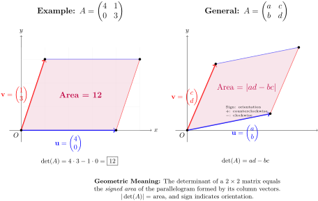
For a \(2 \times 2\) matrix \(A = \begin{pmatrix} a \amp c \\ b \amp d \end{pmatrix}\text{,}\) the absolute value \(|\det(A)| = |ad - bc|\) gives the area of the parallelogram formed by the vectors \(\mathbf{u} = \begin{pmatrix} a \\ b \end{pmatrix}\) and \(\mathbf{v} = \begin{pmatrix} c \\ d \end{pmatrix}\text{.}\)
Example 3.2.14. Area of a Parallelogram in 2D.
Consider the matrix \(A = \begin{pmatrix} 4 \amp 1 \\ 0 \amp 3 \end{pmatrix}\text{.}\) The column vectors are \(\mathbf{u} = \begin{pmatrix} 4 \\ 0 \end{pmatrix}\) and \(\mathbf{v} = \begin{pmatrix} 1 \\ 3 \end{pmatrix}\text{.}\)
Shows how the determinant det(A) = ad - bc equals the area of the parallelogram formed by column vectors.
Figure 3.2.15. The Determinant as the Area of a Parallelogram
The determinant is:
\begin{equation*} \det(A) = 4 \cdot 3 - 1 \cdot 0 = 12 \end{equation*}
So the area of the parallelogram is \(|\det(A)| = 12\) square units.
Insight 3.2.16.
Key Insight: The sign of the determinant tells us about orientation. If \(\det(A) > 0\text{,}\) the vectors \(\mathbf{u}\) and \(\mathbf{v}\) follow a counterclockwise orientation. If \(\det(A) < 0\text{,}\) they follow a clockwise orientation.

Subsubsection 3.2.3.2 3D Case: Volume of a Parallelepiped

For a \(3 \times 3\) matrix \(A = \begin{pmatrix} a_1 \amp b_1 \amp c_1 \\ a_2 \amp b_2 \amp c_2 \\ a_3 \amp b_3 \amp c_3 \end{pmatrix}\text{,}\) the absolute value \(|\det(A)|\) gives the volume of the parallelepiped formed by the three column vectors.
Example 3.2.17. Volume of a Parallelepiped in 3D.
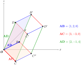
Consider the matrix from the figure:
\begin{equation*} A = \begin{pmatrix} 1 \amp 3 \amp 2 \\ 2 \amp -3 \amp -1 \\ 0 \amp 0 \amp 4 \end{pmatrix} \end{equation*}
This gives us three vectors: \(\mathbf{u} = \langle 1, 2, 0 \rangle\text{,}\) \(\mathbf{v} = \langle 3, -3, 0 \rangle\text{,}\) and \(\mathbf{w} = \langle 2, -1, 4 \rangle\text{.}\)
A parallelepiped in 3D coordinate system
Figure 3.2.18. Parallelepiped formed by three vectors in 3D space
Calculate the determinant:
We can verify this is correct by computing:
\begin{align*} \det(A) \amp = 1 \cdot \begin{vmatrix} -3 \amp -1 \\ 0 \amp 4 \end{vmatrix} - 3 \cdot \begin{vmatrix} 2 \amp -1 \\ 0 \amp 4 \end{vmatrix} + 2 \cdot \begin{vmatrix} 2 \amp -3 \\ 0 \amp 0 \end{vmatrix}\\ \amp = 1(-12 - 0) - 3(8 - 0) + 2(0 - 0)\\ \amp = -12 - 24 + 0 = -36 \end{align*}
Therefore, the volume is \(|\det(A)| = 36\) cubic units.
The geometric interpretation extends to higher dimensions, though we cannot visualize it. For an \(n \times n\) matrix, \(|\det(A)|\) gives the \(n\)-dimensional "hypervolume" of the parallelepiped formed by the \(n\) column vectors.

Activity 3.2.4. Exploring Geometric Determinants.

Use the geometric interpretation to understand determinants better.
(a)
Find the area of the parallelogram formed by vectors \(\mathbf{u} = \langle 2, 1 \rangle\) and \(\mathbf{v} = \langle 3, 4 \rangle\text{.}\)
Hint.
Form a \(2 \times 2\) matrix with these vectors as columns and compute its determinant.
(b)
What happens to the area when you swap the two vectors (i.e., consider \(\mathbf{v}\) and \(\mathbf{u}\) instead)? What changes?
(c)
Find the volume of the parallelepiped formed by \(\mathbf{a} = \langle 1, 0, 0 \rangle\text{,}\) \(\mathbf{b} = \langle 2, 3, 0 \rangle\text{,}\) and \(\mathbf{c} = \langle 1, 1, 5 \rangle\text{.}\)