Section 4.2 Subspaces of \(\mathbb{R}^n\)

Why Study Subspaces?
Understanding subspaces is one of the most important steps in developing mathematical maturity and algebraic thinking. Subspaces reveal the hidden structure within vector spaces and provide a framework for solving complex problems by breaking them down into manageable pieces.
Intellectual and Mathematical Development:
  • Abstraction and Generalization: Subspaces teach us to recognize common patterns across different mathematical objects. The solution set of a homogeneous system, the span of vectors, and the null space of a matrix all share the same fundamental structure—they are all subspaces. This ability to see unity in diversity is a hallmark of mathematical sophistication.
  • Structural Thinking: Rather than viewing vectors as isolated objects, subspaces help us understand how sets of vectors relate to one another and form coherent structures. This structural perspective is essential not only in advanced mathematics but also in fields like data science, physics, and engineering.
  • Problem Decomposition: Many complex problems can be solved by decomposing a vector space into smaller, more manageable subspaces. For example, in solving differential equations or analyzing signal processing problems, we often work within specific subspaces that capture the essential features of the problem.
  • Foundation for Advanced Topics: Subspaces are the building blocks for understanding eigenspaces, orthogonal decompositions, the fundamental theorem of linear algebra, and many other advanced concepts. Mastering subspaces now opens doors to deeper mathematical understanding later.
Practical Importance:
  • Understanding Solution Sets: The solution set of a homogeneous linear system \(A\mathbf{x} = \mathbf{0}\) forms a subspace (the null space). Understanding this helps us characterize all solutions systematically.
  • Data Analysis: In machine learning and statistics, subspaces represent lower-dimensional manifolds in high-dimensional data. Principal Component Analysis (PCA) finds subspaces that capture the most important variations in data.
  • Computer Graphics: Subspaces represent planes, lines, and other geometric objects used in 3D modeling and animation.

Subsection 4.2.1 Definition and Basic Properties

Definition 4.2.1. Subspace.

A subset \(W\) of a vector space \(V\) is called a subspace of \(V\) if \(W\) is itself a vector space under the same operations of addition and scalar multiplication defined on \(V\text{.}\)
Equivalently, \(W\) is a subspace of \(V\) if and only if the following three conditions hold:
  1. Contains the zero vector: \(\mathbf{0} \in W\)
  2. Closed under addition: If \(\mathbf{u}, \mathbf{v} \in W\text{,}\) then \(\mathbf{u} + \mathbf{v} \in W\)
  3. Closed under scalar multiplication: If \(\mathbf{u} \in W\) and \(c \in \mathbb{R}\text{,}\) then \(c\mathbf{u} \in W\)
Why These Three Conditions? These are the minimal conditions needed to ensure that \(W\) inherits the vector space structure from \(V\text{.}\) The other vector space axioms (associativity, commutativity, distributivity, etc.) are automatically satisfied because they hold in \(V\text{.}\)

Insight 4.2.2. The Subspace Test.

To verify that a set \(W\) is a subspace, we only need to check three things:
  1. Is \(\mathbf{0} \in W\text{?}\)
  2. Is \(W\) closed under addition?
  3. Is \(W\) closed under scalar multiplication?
This is much easier than checking all ten vector space axioms!

Geometric Visualization of Subspaces.

Subspaces have beautiful geometric interpretations. In \(\mathbb{R}^2\) and \(\mathbb{R}^3\text{,}\) we can visualize every possible subspace. Key insight: A subspace must always pass through the origin because it must contain the zero vector.
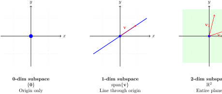
Figure 4.2.3. All subspaces of \(\mathbb{R}^2\)
In \(\mathbb{R}^2\text{,}\) there are exactly three types of subspaces:
  • 0-dimensional: \(\{\mathbf{0}\}\) — the trivial subspace containing only the origin
  • 1-dimensional: Lines through the origin — \(\operatorname{span}\{\mathbf{v}\}\) for any non-zero vector \(\mathbf{v}\)
  • 2-dimensional: \(\mathbb{R}^2\) itself — the entire plane
Note: A line not passing through the origin is not a subspace (it doesn’t contain \(\mathbf{0}\)).
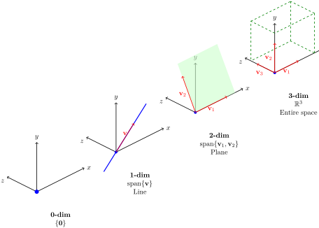
Figure 4.2.4. All subspaces of \(\mathbb{R}^3\)
In \(\mathbb{R}^3\text{,}\) there are exactly four types of subspaces:
  • 0-dimensional: \(\{\mathbf{0}\}\) — just the origin
  • 1-dimensional: Lines through the origin — \(\operatorname{span}\{\mathbf{v}\}\)
  • 2-dimensional: Planes through the origin — \(\operatorname{span}\{\mathbf{v}_1, \mathbf{v}_2\}\) where \(\mathbf{v}_1, \mathbf{v}_2\) are linearly independent
  • 3-dimensional: \(\mathbb{R}^3\) itself — the entire space
Insight 4.2.5. The Pattern of Subspaces.
  • Nested structure: Subspaces form a hierarchy. In \(\mathbb{R}^3\text{:}\) \(\{\mathbf{0}\}\) ⊆ (lines) ⊆ (planes) ⊆ \(\mathbb{R}^3\text{.}\) Each level adds one dimension.
  • Origin is essential: Every subspace must contain \(\mathbf{0}\text{.}\) This is why "a plane 3 units above the xy-plane" is not a subspace—it doesn’t pass through the origin.
  • Subspaces are determined by spanning sets:
    • 1D subspace = \(\operatorname{span}\{\)one non-zero vector\(\}\)
    • 2D subspace = \(\operatorname{span}\{\)two linearly independent vectors\(\}\)
    • \(k\)D subspace = \(\operatorname{span}\{k\) linearly independent vectors\(\}\)
  • General pattern in \(\mathbb{R}^n\text{:}\) The subspaces of \(\mathbb{R}^n\) have dimensions 0, 1, 2, ..., \(n\text{.}\) A \(k\)-dimensional subspace is spanned by exactly \(k\) linearly independent vectors.

Subsection 4.2.2 Examples of Subspaces

Example 4.2.6. Trivial Subspaces.

Every vector space \(V\) has two trivial subspaces:
  1. \(V\) itself is a subspace of \(V\)
  2. The set \(\{\mathbf{0}\}\) containing only the zero vector is a subspace of \(V\)
Solution.
Verification for \(\{\mathbf{0}\}\text{:}\)
  1. \(\mathbf{0} \in \{\mathbf{0}\}\)
  2. If \(\mathbf{u}, \mathbf{v} \in \{\mathbf{0}\}\text{,}\) then \(\mathbf{u} = \mathbf{v} = \mathbf{0}\text{,}\) so \(\mathbf{u} + \mathbf{v} = \mathbf{0} + \mathbf{0} = \mathbf{0} \in \{\mathbf{0}\}\)
  3. If \(\mathbf{u} \in \{\mathbf{0}\}\text{,}\) then \(\mathbf{u} = \mathbf{0}\text{,}\) so \(c\mathbf{u} = c\mathbf{0} = \mathbf{0} \in \{\mathbf{0}\}\)

Example 4.2.7. A Line Through the Origin.

Let \(W = \left\{t\begin{bmatrix}2\\1\end{bmatrix} \mid t \in \mathbb{R}\right\}\) be the set of all scalar multiples of the vector \(\begin{bmatrix}2\\1\end{bmatrix}\text{.}\) Show that \(W\) is a subspace of \(\mathbb{R}^2\text{.}\)
Solution.
We verify the three conditions:
  1. Contains zero: When \(t = 0\text{,}\) we get \(0\begin{bmatrix}2\\1\end{bmatrix} = \begin{bmatrix}0\\0\end{bmatrix} = \mathbf{0}\text{,}\) so \(\mathbf{0} \in W\)
  2. Closed under addition: Let \(\mathbf{u} = s\begin{bmatrix}2\\1\end{bmatrix}\) and \(\mathbf{v} = t\begin{bmatrix}2\\1\end{bmatrix}\) be in \(W\text{.}\) Then
    \begin{equation*} \mathbf{u} + \mathbf{v} = s\begin{bmatrix}2\\1\end{bmatrix} + t\begin{bmatrix}2\\1\end{bmatrix} = (s+t)\begin{bmatrix}2\\1\end{bmatrix} \end{equation*}
    Since \(s+t \in \mathbb{R}\text{,}\) we have \(\mathbf{u} + \mathbf{v} \in W\)
  3. Closed under scalar multiplication: Let \(\mathbf{u} = t\begin{bmatrix}2\\1\end{bmatrix} \in W\) and \(c \in \mathbb{R}\text{.}\) Then
    \begin{equation*} c\mathbf{u} = c\left(t\begin{bmatrix}2\\1\end{bmatrix}\right) = (ct)\begin{bmatrix}2\\1\end{bmatrix} \end{equation*}
    Since \(ct \in \mathbb{R}\text{,}\) we have \(c\mathbf{u} \in W\)
Geometric Interpretation: \(W\) represents a line through the origin in \(\mathbb{R}^2\) with direction vector \(\begin{bmatrix}2\\1\end{bmatrix}\text{.}\) Any line through the origin in \(\mathbb{R}^n\) is a subspace.

Example 4.2.8. A Plane Through the Origin.

Let \(W = \left\{s\begin{bmatrix}1\\0\\1\end{bmatrix} + t\begin{bmatrix}0\\1\\1\end{bmatrix} \mid s, t \in \mathbb{R}\right\}\text{.}\) Show that \(W\) is a subspace of \(\mathbb{R}^3\text{.}\)
Solution.
We verify the three conditions:
  1. Contains zero: When \(s = t = 0\text{,}\) we get \(\mathbf{0} \in W\)
  2. Closed under addition: Let \(\mathbf{u} = s_1\begin{bmatrix}1\\0\\1\end{bmatrix} + t_1\begin{bmatrix}0\\1\\1\end{bmatrix}\) and \(\mathbf{v} = s_2\begin{bmatrix}1\\0\\1\end{bmatrix} + t_2\begin{bmatrix}0\\1\\1\end{bmatrix}\) be in \(W\text{.}\) Then
    \begin{align*} \mathbf{u} + \mathbf{v} &= \left(s_1\begin{bmatrix}1\\0\\1\end{bmatrix} + t_1\begin{bmatrix}0\\1\\1\end{bmatrix}\right) + \left(s_2\begin{bmatrix}1\\0\\1\end{bmatrix} + t_2\begin{bmatrix}0\\1\\1\end{bmatrix}\right)\\ &= (s_1+s_2)\begin{bmatrix}1\\0\\1\end{bmatrix} + (t_1+t_2)\begin{bmatrix}0\\1\\1\end{bmatrix} \end{align*}
    Since \(s_1+s_2, t_1+t_2 \in \mathbb{R}\text{,}\) we have \(\mathbf{u} + \mathbf{v} \in W\)
  3. Closed under scalar multiplication: Let \(\mathbf{u} = s\begin{bmatrix}1\\0\\1\end{bmatrix} + t\begin{bmatrix}0\\1\\1\end{bmatrix} \in W\) and \(c \in \mathbb{R}\text{.}\) Then
    \begin{equation*} c\mathbf{u} = c\left(s\begin{bmatrix}1\\0\\1\end{bmatrix} + t\begin{bmatrix}0\\1\\1\end{bmatrix}\right) = (cs)\begin{bmatrix}1\\0\\1\end{bmatrix} + (ct)\begin{bmatrix}0\\1\\1\end{bmatrix} \end{equation*}
    Since \(cs, ct \in \mathbb{R}\text{,}\) we have \(c\mathbf{u} \in W\)
Geometric Interpretation: \(W = \operatorname{span}\left\{\begin{bmatrix}1\\0\\1\end{bmatrix}, \begin{bmatrix}0\\1\\1\end{bmatrix}\right\}\) represents a plane through the origin in \(\mathbb{R}^3\text{.}\) Any plane through the origin in \(\mathbb{R}^n\) is a subspace.

Example 4.2.9. Solution Set of a Homogeneous System.

Let \(A\) be an \(m \times n\) matrix, and let \(W = \{\mathbf{x} \in \mathbb{R}^n \mid A\mathbf{x} = \mathbf{0}\}\) be the solution set of the homogeneous system \(A\mathbf{x} = \mathbf{0}\text{.}\) Show that \(W\) is a subspace of \(\mathbb{R}^n\text{.}\)
Solution.
  1. Contains zero: \(A\mathbf{0} = \mathbf{0}\text{,}\) so \(\mathbf{0} \in W\)
  2. Closed under addition: If \(\mathbf{u}, \mathbf{v} \in W\text{,}\) then \(A\mathbf{u} = \mathbf{0}\) and \(A\mathbf{v} = \mathbf{0}\text{.}\) Therefore,
    \begin{equation*} A(\mathbf{u} + \mathbf{v}) = A\mathbf{u} + A\mathbf{v} = \mathbf{0} + \mathbf{0} = \mathbf{0} \end{equation*}
    so \(\mathbf{u} + \mathbf{v} \in W\)
  3. Closed under scalar multiplication: If \(\mathbf{u} \in W\) and \(c \in \mathbb{R}\text{,}\) then \(A\mathbf{u} = \mathbf{0}\text{.}\) Therefore,
    \begin{equation*} A(c\mathbf{u}) = c(A\mathbf{u}) = c\mathbf{0} = \mathbf{0} \end{equation*}
    so \(c\mathbf{u} \in W\)
Important Note: This subspace \(W\) is called the null space or kernel of the matrix \(A\text{,}\) denoted \(\operatorname{Null}(A)\) or \(\ker(A)\text{.}\) We will study this in detail in the next section.

Example 4.2.10. The Span of Vectors is a Subspace.

Let \(S = \{v_1, v_2, \ldots, v_k\}\) be a set of vectors in \(\mathbb{R}^n\text{.}\) Show that \(W = \operatorname{span}(S)\) is a subspace of \(\mathbb{R}^n\text{.}\)
Solution.
This generalizes what we proved in the span section. Recall that
\begin{equation*} \operatorname{span}(S) = \{c_1v_1 + c_2v_2 + \cdots + c_kv_k \mid c_i \in \mathbb{R}\} \end{equation*}
  1. Contains zero: \(\mathbf{0} = 0v_1 + 0v_2 + \cdots + 0v_k \in \operatorname{span}(S)\)
  2. Closed under addition: We showed this in the span section ✓
  3. Closed under scalar multiplication: We showed this in the span section ✓
Key Insight: Every span is a subspace. This is one of the most important connections in linear algebra. It means that whenever we talk about the span of vectors, we are automatically talking about a subspace.

Example 4.2.11. A Set That Is NOT a Subspace.

Let \(W = \left\{\begin{bmatrix}x\\y\end{bmatrix} \in \mathbb{R}^2 \mid x + y = 1\right\}\text{.}\) Show that \(W\) is not a subspace of \(\mathbb{R}^2\text{.}\)
Solution.
Geometric Interpretation: \(W\) is a line in \(\mathbb{R}^2\text{,}\) but it does not pass through the origin (it’s the line \(x + y = 1\)).
To show \(W\) is not a subspace, we only need to find one condition that fails:
Test 1: Contains zero? The zero vector is \(\begin{bmatrix}0\\0\end{bmatrix}\text{.}\) But \(0 + 0 = 0 \neq 1\text{,}\) so \(\mathbf{0} \notin W\)
Since the first condition fails, \(W\) is not a subspace.
Alternative Test - Closure under addition: Even if we didn’t check the zero vector, we could show \(W\) is not closed under addition. Let \(\mathbf{u} = \begin{bmatrix}1\\0\end{bmatrix}\) and \(\mathbf{v} = \begin{bmatrix}0\\1\end{bmatrix}\text{.}\) Both are in \(W\) since \(1+0=1\) and \(0+1=1\text{.}\) But
\begin{equation*} \mathbf{u} + \mathbf{v} = \begin{bmatrix}1\\1\end{bmatrix} \end{equation*}
and \(1 + 1 = 2 \neq 1\text{,}\) so \(\mathbf{u} + \mathbf{v} \notin W\)
Lesson: A set that looks "linear" (like a line) is not automatically a subspace. The crucial requirement is that it must pass through the origin and be closed under the vector space operations.

Subsection 4.2.3 Important Theorem

Proof.

We need to show two things:
  1. \(\operatorname{span}(S)\) is a subspace containing \(S\) (already proved)
  2. Any other subspace \(W\) containing \(S\) must contain \(\operatorname{span}(S)\)
For part 2: Let \(W\) be a subspace with \(v_1, v_2, \ldots, v_k \in W\text{.}\) We need to show \(\operatorname{span}(S) \subseteq W\text{.}\)
Take any vector \(\mathbf{u} \in \operatorname{span}(S)\text{.}\) Then \(\mathbf{u} = c_1v_1 + c_2v_2 + \cdots + c_kv_k\) for some scalars \(c_i\text{.}\)
Since \(W\) is a subspace:
  • Each \(v_i \in W\) (by assumption)
  • Each \(c_iv_i \in W\) (closure under scalar multiplication)
  • \(c_1v_1 + c_2v_2 + \cdots + c_kv_k \in W\) (closure under addition)
Therefore \(\mathbf{u} \in W\text{,}\) which shows \(\operatorname{span}(S) \subseteq W\text{.}\)
Significance: This theorem tells us that span is not just a subspace—it’s the most economical subspace containing the given vectors. This makes span the natural tool for constructing subspaces from a given set of vectors.

Activity 4.2.1.

Let \(A\) be an \(m\times n\) matrix.
(a)
Prove that the solution set of the homogeneous system \(A\mathbf{x} = \mathbf{0}\) is a subspace of \(\mathbb{R}^n\text{.}\)
Solution.
We need to verify the three conditions of the subspace test:
  1. Contains zero: The zero vector \(\mathbf{0}\) satisfies \(A\mathbf{0} = \mathbf{0}\text{,}\) so \(\mathbf{0}\) is in the solution set.
  2. Closed under addition: Let \(\mathbf{u}\) and \(\mathbf{v}\) be two solutions to \(A\mathbf{x} = \mathbf{0}\text{.}\) Then \(A\mathbf{u} = \mathbf{0}\) and \(A\mathbf{v} = \mathbf{0}\text{.}\) Therefore,
    \begin{equation*} A(\mathbf{u} + \mathbf{v}) = A\mathbf{u} + A\mathbf{v} = \mathbf{0} + \mathbf{0} = \mathbf{0} \end{equation*}
    Thus, \(\mathbf{u} + \mathbf{v}\) is also a solution.
  3. Closed under scalar multiplication: Let \(\mathbf{u}\) be a solution to \(A\mathbf{x} = \mathbf{0}\) and let \(c \in \mathbb{R}\text{.}\) Then,
    \begin{equation*} A(c\mathbf{u}) = c(A\mathbf{u}) = c\mathbf{0} = \mathbf{0} \end{equation*}
    Thus, \(c\mathbf{u}\) is also a solution.
(b)
Suppose that \(\mathbf{b}\neq \mathbf{0}\text{.}\) Prove that the solution set of the homogeneous system \(A\mathbf{x} = \mathbf{b}\) is not a subspace of \(\mathbb{R}^n\text{.}\)