Section 7.7 Application III: Conic Sections, Quadric Surfaces, and Positive Definite Matrices

In the previous sections we saw how orthogonal diagonalization transforms a quadratic form \(\mathbf{x}^TA\mathbf{x}\) into a sum of squares \(\lambda_1 y_1^2 + \cdots + \lambda_n y_n^2\text{.}\) When we set a quadratic form equal to a constant, we obtain a geometric curve or surface: in two dimensions we get the classical conic sections (ellipses, hyperbolas, parabolas), and in three dimensions we get quadric surfaces.
We begin with a thorough study of conic sections in \(\mathbb{R}^2\text{,}\) since these are both more familiar and easier to visualize. The key idea—using eigenvalues to eliminate cross terms and identify the curve type—extends directly to three dimensions. We then classify the six basic types of quadric surfaces, use eigenvalue methods to identify surfaces whose equations contain cross terms, and conclude with the important concept of positive definite matrices.

Subsection 7.7.1 Conic Sections in \(\mathbb{R}^2\)

A conic section (or simply a conic) is the set of all points \((x, y)\) in \(\mathbb{R}^2\) satisfying a general second-degree equation
\begin{equation*} Ax^2 + Bxy + Cy^2 + Dx + Ey + F = 0, \end{equation*}
where at least one of \(A, B, C\) is nonzero. The name comes from the fact that these curves can all be obtained by slicing a double cone with a plane.
When the equation is in standard position (centered at the origin and aligned with the coordinate axes, with no \(xy\)-term), the four fundamental types are:

The Four Standard Conic Sections.

  1. Ellipse:
    \begin{equation*} \frac{x^2}{a^2} + \frac{y^2}{b^2} = 1 \quad (a, b > 0) \end{equation*}
    A closed, oval-shaped curve. When \(a = b\text{,}\) it is a circle.
  2. Hyperbola:
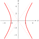
    \begin{equation*} \frac{x^2}{a^2} - \frac{y^2}{b^2} = 1 \quad (a, b > 0) \end{equation*}
    Two separate branches opening along the \(x\)-axis, with asymptotes \(y = \pm \tfrac{b}{a}x\text{.}\)
  3. Parabola:
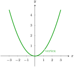
    \begin{equation*} y = ax^2 \quad (a \neq 0) \end{equation*}
    An open curve with a single vertex. It opens upward if \(a > 0\) and downward if \(a < 0\text{.}\)
  4. Degenerate cases: A single point, a pair of intersecting lines, a pair of parallel lines, or the empty set. These arise when the conic "collapses."
described in detail following the image
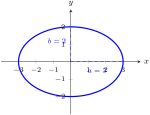
An ellipse centered at the origin with semi-major axis 3 along the x-axis and semi-minor axis 2 along the y-axis.
(a) Ellipse: \(\frac{x^2}{9}+\frac{y^2}{4}=1\)
described in detail following the image
A hyperbola with two branches opening left and right, with asymptotes y = 3x/2 and y = -3x/2 shown as dashed lines.
(b) Hyperbola: \(\frac{x^2}{4}-\frac{y^2}{9}=1\)
described in detail following the image
A parabola opening upward with vertex at the origin.
(c) Parabola: \(y = \frac{1}{2}x^2\)
Figure 7.7.1. The three standard types of conic sections, shown in standard position.
The connection to linear algebra comes from writing the quadratic part of the equation in matrix form. For the general second-degree equation \(Ax^2 + Bxy + Cy^2 = k\) (ignoring linear and constant terms for now), we can write
\begin{equation*} \begin{bmatrix} x \amp y \end{bmatrix} \begin{bmatrix} A \amp B/2 \\ B/2 \amp C \end{bmatrix} \begin{bmatrix} x \\ y \end{bmatrix} = k, \end{equation*}
or equivalently \(\mathbf{x}^T M \mathbf{x} = k\text{,}\) where \(M\) is a \(2 \times 2\) symmetric matrix. The eigenvalues of \(M\) determine the type of conic:

Insight 7.7.2. Classifying Conics by Eigenvalues.

For the equation \(\mathbf{x}^TM\mathbf{x} = k\) with \(M\) a \(2 \times 2\) symmetric matrix having eigenvalues \(\lambda_1\) and \(\lambda_2\text{:}\)
  • \(\lambda_1, \lambda_2\) both positive (and \(k > 0\)): ellipse
  • \(\lambda_1, \lambda_2\) have opposite signs (and \(k \neq 0\)): hyperbola
  • \(\lambda_1, \lambda_2\) both positive (and \(k = 0\)): single point (degenerate ellipse)
  • \(\lambda_1, \lambda_2\) have opposite signs (and \(k = 0\)): pair of intersecting lines (degenerate hyperbola)
This is a direct consequence of the Principal Axis Theorem: after the substitution \(\mathbf{x} = P\mathbf{y}\text{,}\) the equation becomes \(\lambda_1 y_1^2 + \lambda_2 y_2^2 = k\text{,}\) which is in standard form.

Example 7.7.3. Rotation of Axes — Identifying an Ellipse.

Identify and sketch the conic section
\begin{equation*} 5x^2 - 4xy + 8y^2 = 36. \end{equation*}
Solution.
Step 1: Write the equation in matrix form. The associated symmetric matrix is
\begin{equation*} M = \begin{bmatrix} 5 \amp -2 \\ -2 \amp 8 \end{bmatrix}. \end{equation*}
(The cross term \(-4xy\) contributes \(-2\) to both off-diagonal entries.)
Step 2: Find eigenvalues. The characteristic polynomial is
\begin{equation*} \det(M - \lambda I) = (5-\lambda)(8-\lambda) - 4 = \lambda^2 - 13\lambda + 36 = (\lambda - 4)(\lambda - 9) = 0. \end{equation*}
So \(\lambda_1 = 4\) and \(\lambda_2 = 9\text{.}\)
Step 3: Find eigenvectors. For \(\lambda_1 = 4\text{:}\) solving \((M - 4I)\mathbf{v} = \mathbf{0}\) gives \(\mathbf{v}_1 = \begin{bmatrix} 2 \\ 1 \end{bmatrix}\text{.}\) For \(\lambda_2 = 9\text{:}\) solving \((M - 9I)\mathbf{v} = \mathbf{0}\) gives \(\mathbf{v}_2 = \begin{bmatrix} -1 \\ 2 \end{bmatrix}\text{.}\) Normalizing:
\begin{equation*} \mathbf{u}_1 = \frac{1}{\sqrt{5}}\begin{bmatrix} 2 \\ 1 \end{bmatrix}, \qquad \mathbf{u}_2 = \frac{1}{\sqrt{5}}\begin{bmatrix} -1 \\ 2 \end{bmatrix}. \end{equation*}
Step 4: Change coordinates. Let \(\mathbf{x} = P\mathbf{y}\) where \(P = [\mathbf{u}_1 \mid \mathbf{u}_2]\text{.}\) The equation becomes
\begin{equation*} 4y_1^2 + 9y_2^2 = 36, \qquad \text{i.e.,} \qquad \frac{y_1^2}{9} + \frac{y_2^2}{4} = 1. \end{equation*}
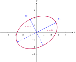
This is an ellipse with semi-axes \(a = 3\) and \(b = 2\) in the rotated coordinate system. The principal axes of the ellipse are along the eigenvectors \(\mathbf{u}_1\) and \(\mathbf{u}_2\text{.}\)
described in detail following the image
A tilted ellipse in the xy-plane with two rotated coordinate axes (eigenvector directions) shown, demonstrating rotation of axes that eliminates the cross term.
Figure 7.7.4. The ellipse \(5x^2 - 4xy + 8y^2 = 36\) shown in both the original \(xy\)-coordinates and the rotated \(y_1 y_2\)-coordinates. The principal axes (eigenvectors) are shown in blue.

Example 7.7.5. Rotation of Axes — Identifying a Hyperbola.

Identify and sketch the conic section
\begin{equation*} x^2 + 4xy + y^2 = 6. \end{equation*}
Solution.
Step 1: Write the equation in matrix form. The associated symmetric matrix is
\begin{equation*} M = \begin{bmatrix} 1 \amp 2 \\ 2 \amp 1 \end{bmatrix}. \end{equation*}
Step 2: Find eigenvalues.
\begin{equation*} \det(M - \lambda I) = (1 - \lambda)^2 - 4 = \lambda^2 - 2\lambda - 3 = (\lambda - 3)(\lambda + 1) = 0. \end{equation*}
So \(\lambda_1 = 3\) and \(\lambda_2 = -1\text{.}\) Since the eigenvalues have opposite signs, the curve is a hyperbola.
Step 3: Find eigenvectors and change coordinates. For \(\lambda_1 = 3\text{:}\) \(\mathbf{u}_1 = \frac{1}{\sqrt{2}}\begin{bmatrix} 1 \\ 1 \end{bmatrix}\text{.}\) For \(\lambda_2 = -1\text{:}\) \(\mathbf{u}_2 = \frac{1}{\sqrt{2}}\begin{bmatrix} -1 \\ 1 \end{bmatrix}\text{.}\)
The equation becomes
\begin{equation*} 3y_1^2 - y_2^2 = 6, \qquad \text{i.e.,} \qquad \frac{y_1^2}{2} - \frac{y_2^2}{6} = 1. \end{equation*}
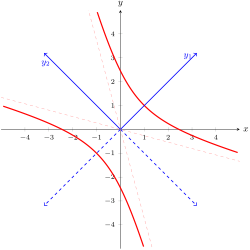
This is a hyperbola with \(a = \sqrt{2}\) and \(b = \sqrt{6}\) in the rotated coordinates, opening along the \(y_1\)-direction (the direction of \(\frac{1}{\sqrt{2}}(1, 1)^T\text{,}\) which is the line \(y = x\)).
described in detail following the image
A rotated hyperbola in the xy-plane with two branches opening along the direction y=x. The rotated coordinate axes and asymptotes are shown.
Figure 7.7.6. The hyperbola \(x^2 + 4xy + y^2 = 6\) with the rotated axes along the eigenvector directions. The branches open along \(y_1\) (the line \(y = x\)) and the asymptotes are along \(y_2\) (the line \(y = -x\)).
The discriminant of the general conic \(Ax^2 + Bxy + Cy^2 = k\) provides a quick classification without computing eigenvalues:

Discriminant Test for Conics.

For the equation \(Ax^2 + Bxy + Cy^2 = k\) (with \(k \neq 0\)), the discriminant is \(\Delta = B^2 - 4AC\text{:}\)
  • \(\Delta < 0\text{:}\) the curve is an ellipse (or a circle if \(A = C\) and \(B = 0\))
  • \(\Delta > 0\text{:}\) the curve is a hyperbola
  • \(\Delta = 0\text{:}\) the curve is a parabola (or degenerate)
This follows from the fact that \(\Delta = B^2 - 4AC = -4\det(M)\text{,}\) and \(\det(M) = \lambda_1\lambda_2\text{.}\) So \(\Delta < 0\) means \(\lambda_1\lambda_2 > 0\) (same sign), and \(\Delta > 0\) means \(\lambda_1\lambda_2 < 0\) (opposite signs).

Example 7.7.7. Quick Classification Using the Discriminant.

Classify each conic without computing eigenvalues:
  1. \(\displaystyle 3x^2 + 2xy + 3y^2 = 8\)
  2. \(\displaystyle x^2 - 6xy + y^2 = 4\)
  3. \(\displaystyle x^2 + 2xy + y^2 = 1\)
Solution.
  1. \(\Delta = 2^2 - 4(3)(3) = 4 - 36 = -32 < 0\text{:}\) ellipse.
  2. \(\Delta = (-6)^2 - 4(1)(1) = 36 - 4 = 32 > 0\text{:}\) hyperbola.
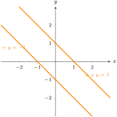
  3. \(\Delta = 2^2 - 4(1)(1) = 4 - 4 = 0\text{:}\) degenerate (a pair of parallel lines: \((x+y)^2 = 1\text{,}\) i.e., \(x + y = \pm 1\)).
described in detail following the image
Two parallel lines: x+y=1 and x+y=-1, shown in the xy-plane.
(a) Parallel lines: \((x+y)^2=1\)
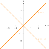
described in detail following the image
Two lines crossing at the origin: y=x and y=-x.
(b) Intersecting lines: \(x^2-y^2=0\)
Figure 7.7.8. Degenerate conic sections: when the quadratic form has a zero eigenvalue, the conic "collapses." Left: a pair of parallel lines from \((x+y)^2=1\text{.}\) Right: a pair of intersecting lines from \(x^2 - y^2 = 0\text{.}\)

Subsection 7.7.2 From Conics to Quadric Surfaces

Just as conic sections are defined by second-degree equations in two variables, quadric surfaces in \(\mathbb{R}^3\) are defined by second-degree equations in three variables. The classification strategy is the same: write the quadratic part as \(\mathbf{x}^TA\mathbf{x}\text{,}\) diagonalize \(A\text{,}\) and read off the surface type from the signs of the eigenvalues. Instead of three types of nondegenerate conics, there are now six basic types of quadric surfaces—the natural three-dimensional analogues.

The Six Basic Quadric Surfaces.

  1. Ellipsoid:
    \begin{equation*} \frac{x^2}{a^2} + \frac{y^2}{b^2} + \frac{z^2}{c^2} = 1 \end{equation*}
    All cross-sections are ellipses (or circles when two semi-axes are equal). The surface is a bounded, egg-shaped solid. When \(a = b = c\text{,}\) it is a sphere. (3D analogue of the ellipse.)
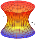
  2. Hyperboloid of one sheet:
    \begin{equation*} \frac{x^2}{a^2} + \frac{y^2}{b^2} - \frac{z^2}{c^2} = 1 \end{equation*}
    Horizontal cross-sections (\(z = k\)) are ellipses; vertical cross-sections through the origin are hyperbolas. The surface looks like a cooling tower—connected in one piece with a "waist."
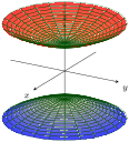
  3. Hyperboloid of two sheets:
    \begin{equation*} -\frac{x^2}{a^2} - \frac{y^2}{b^2} + \frac{z^2}{c^2} = 1 \end{equation*}
    Horizontal cross-sections are ellipses only for \(|z| > c\text{.}\) The surface consists of two separate bowl-shaped pieces opening along the \(z\)-axis. (Both hyperboloid types are 3D analogues of the hyperbola.)
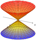
  4. Elliptic cone:
    \begin{equation*} \frac{x^2}{a^2} + \frac{y^2}{b^2} - \frac{z^2}{c^2} = 0 \end{equation*}
    This is the "transition" between the one-sheet and two-sheet hyperboloids. The surface has a vertex at the origin and opens along the \(z\)-axis, with elliptical cross-sections. (3D analogue of the degenerate conic: a pair of intersecting lines.)
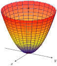
  5. Elliptic paraboloid:
    \begin{equation*} z = \frac{x^2}{a^2} + \frac{y^2}{b^2} \end{equation*}
    Horizontal cross-sections are ellipses; the surface is a bowl opening upward (or downward if \(z\) is negated). This shape appears in satellite dishes and reflectors.
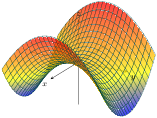
  6. Hyperbolic paraboloid (saddle surface):
    \begin{equation*} z = \frac{x^2}{a^2} - \frac{y^2}{b^2} \end{equation*}
    This surface curves upward in one direction and downward in another, creating a saddle shape (like a Pringles chip). It has no global maximum or minimum. (Both paraboloid types are 3D analogues of the parabola.)
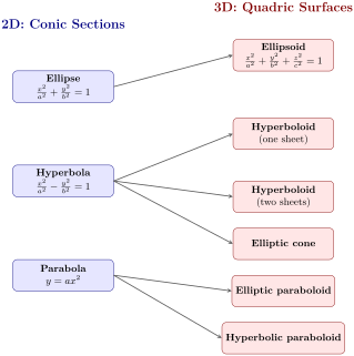
described in detail following the image
A diagram showing the correspondence between conics and quadric surfaces: ellipse maps to ellipsoid, hyperbola maps to hyperboloids, and parabola maps to paraboloids.
Figure 7.7.9. From 2D to 3D: each type of conic section corresponds to one or more types of quadric surfaces. Rotating a conic around an axis of symmetry produces a surface of revolution—a special case of a quadric surface.
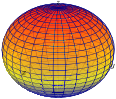
described in detail following the image
A three-dimensional ellipsoid surface.
(a) Ellipsoid: \(\dfrac{x^2}{a^2}+\dfrac{y^2}{b^2}+\dfrac{z^2}{c^2}=1\)
described in detail following the image
A three-dimensional hyperboloid of one sheet surface.
(b) Hyperboloid of one sheet: \(\dfrac{x^2}{a^2}+\dfrac{y^2}{b^2}-\dfrac{z^2}{c^2}=1\)
described in detail following the image
A three-dimensional hyperboloid of two sheets surface with two separate bowl-shaped pieces.
(c) Hyperboloid of two sheets: \(-\dfrac{x^2}{a^2}-\dfrac{y^2}{b^2}+\dfrac{z^2}{c^2}=1\)
described in detail following the image
A three-dimensional elliptic cone surface with vertex at the origin.
(d) Elliptic cone: \(\dfrac{x^2}{a^2}+\dfrac{y^2}{b^2}-\dfrac{z^2}{c^2}=0\)
described in detail following the image
A three-dimensional elliptic paraboloid (bowl shape) opening upward.
(e) Elliptic paraboloid: \(z=\dfrac{x^2}{a^2}+\dfrac{y^2}{b^2}\)
described in detail following the image
A three-dimensional hyperbolic paraboloid (saddle surface) curving up in one direction and down in another.
(f) Hyperbolic paraboloid: \(z=\dfrac{x^2}{a^2}-\dfrac{y^2}{b^2}\)
Figure 7.7.10. The six basic types of quadric surfaces.

Insight 7.7.11. Reading Surface Type from Eigenvalues.

The type of a quadric surface \(\mathbf{x}^TA\mathbf{x} = c\) is determined by the signs of the eigenvalues of \(A\) and the constant \(c\text{.}\) This is a direct generalization of the conic section classification from Insight 7.7.2:
  • All eigenvalues positive (\(c > 0\)): ellipsoid.
  • Two positive, one negative (\(c > 0\)): hyperboloid of one sheet.
  • One positive, two negative (\(c > 0\)), or equivalently two positive, one negative (\(c < 0\)): hyperboloid of two sheets.
  • Two positive, one negative (\(c = 0\)): elliptic cone.
  • All eigenvalues positive but one is zero: elliptic paraboloid (after appropriate interpretation).
  • One positive, one negative, one zero: hyperbolic paraboloid (after appropriate interpretation).

Example 7.7.12. Graphing an Ellipsoid.

Describe and sketch the quadric surface
\begin{equation*} \frac{x^2}{6^2} + \frac{y^2}{3^2} + \frac{z^2}{2^2} = 1. \end{equation*}
Solution.
This equation has the standard form of an ellipsoid with semi-axes \(a = 6\text{,}\) \(b = 3\text{,}\) and \(c = 2\text{.}\)
To understand its shape, we examine cross-sections (just as we did for conics, but now slicing with coordinate planes):
  • Setting \(z = 0\text{:}\) \(\dfrac{x^2}{36} + \dfrac{y^2}{9} = 1\text{,}\) an ellipse in the \(xy\)-plane with semi-axes \(6\) and \(3\text{.}\)
  • Setting \(y = 0\text{:}\) \(\dfrac{x^2}{36} + \dfrac{z^2}{4} = 1\text{,}\) an ellipse in the \(xz\)-plane with semi-axes \(6\) and \(2\text{.}\)
  • Setting \(x = 0\text{:}\) \(\dfrac{y^2}{9} + \dfrac{z^2}{4} = 1\text{,}\) an ellipse in the \(yz\)-plane with semi-axes \(3\) and \(2\text{.}\)
The surface is bounded, enclosing the region \(-6 \le x \le 6\text{,}\) \(-3 \le y \le 3\text{,}\) \(-2 \le z \le 2\text{.}\) It is longest along the \(x\)-axis and shortest along the \(z\)-axis.

Subsection 7.7.3 Using Orthogonal Diagonalization to Identify Quadric Surfaces

When a quadratic equation in \(x, y, z\) contains cross terms (\(xy\text{,}\) \(xz\text{,}\) or \(yz\)), it is not immediately clear what type of surface we have. The strategy is the same one we used for conics in Subsection 7.7.1: diagonalize the associated symmetric matrix and read off the surface type from the eigenvalues.

Strategy: Rotation of Axes for Quadric Surfaces.

Given a quadratic equation \(\mathbf{x}^TA\mathbf{x} = c\) with cross terms:
  1. Identify the symmetric matrix \(A\text{.}\)
  2. Orthogonally diagonalize \(A = PDP^T\) to find eigenvalues \(\lambda_1, \lambda_2, \lambda_3\text{.}\)
  3. Substitute \(\mathbf{x} = P\mathbf{y}\text{.}\) In the new coordinates, the equation becomes \(\lambda_1 y_1^2 + \lambda_2 y_2^2 + \lambda_3 y_3^2 = c\text{.}\)
  4. Match this standard form to one of the six basic types.

Example 7.7.13. Rotation of Axes — Identifying a Hyperboloid.

Perform a rotation of axes to eliminate the cross term in
\begin{equation*} 5x^2 + 4y^2 + 5z^2 + 8xz - 36 = 0, \end{equation*}
and then identify the type of quadric surface.
Solution.
Step 1: Write the equation in matrix form. The quadratic part is \(5x^2 + 4y^2 + 5z^2 + 8xz\text{.}\) The cross term \(8xz\) contributes \(4\) to both the \((1,3)\) and \((3,1)\) entries. The associated symmetric matrix is
\begin{equation*} A = \begin{bmatrix} 5 \amp 0 \amp 4 \\ 0 \amp 4 \amp 0 \\ 4 \amp 0 \amp 5 \end{bmatrix}. \end{equation*}
The equation is \(\mathbf{x}^TA\mathbf{x} = 36\text{.}\)
Step 2: Find eigenvalues and eigenvectors of \(A\text{.}\)
The eigenvalues are \(\lambda_1 = 1\text{,}\) \(\lambda_2 = 4\text{,}\) and \(\lambda_3 = 9\text{.}\) An orthonormal set of eigenvectors is
\begin{equation*} \mathbf{u}_1 = \frac{1}{\sqrt{2}}\begin{bmatrix} 1 \\ 0 \\ -1 \end{bmatrix}, \quad \mathbf{u}_2 = \begin{bmatrix} 0 \\ 1 \\ 0 \end{bmatrix}, \quad \mathbf{u}_3 = \frac{1}{\sqrt{2}}\begin{bmatrix} 1 \\ 0 \\ 1 \end{bmatrix}. \end{equation*}
Step 3: Change coordinates. Let \(\mathbf{x} = P\mathbf{y}\) where \(P = [\mathbf{u}_1 \mid \mathbf{u}_2 \mid \mathbf{u}_3]\text{.}\) The equation becomes
\begin{equation*} \lambda_1 y_1^2 + \lambda_2 y_2^2 + \lambda_3 y_3^2 = 36, \qquad \text{i.e.,} \qquad y_1^2 + 4y_2^2 + 9y_3^2 = 36. \end{equation*}
Dividing by \(36\text{:}\)
\begin{equation*} \frac{y_1^2}{36} + \frac{y_2^2}{9} + \frac{y_3^2}{4} = 1. \end{equation*}
Step 4: Identify the surface. This is an ellipsoid in the rotated coordinates with semi-axes \(6\text{,}\) \(3\text{,}\) and \(2\) along the \(y_1\)-, \(y_2\)-, and \(y_3\)-axes respectively. The original surface is therefore an ellipsoid whose principal axes are aligned with the eigenvectors of \(A\) rather than the standard coordinate axes.
Example 7.7.14. Rotation of Axes — Identifying a Paraboloid.

Perform a rotation of axes to eliminate the cross terms in
\begin{equation*} f(x,y,z) = x^2 + 4xy + 4xz + y^2 + 4yz + z^2, \end{equation*}
and then sketch the graph of the quadric surface \(f(x,y,z) = 28\text{.}\)
Solution.
Step 1: Write the quadratic form in matrix form. We already found in Example 7.4.8 that
\begin{equation*} A = \begin{bmatrix} 1 \amp 2 \amp 2 \\ 2 \amp 1 \amp 2 \\ 2 \amp 2 \amp 1 \end{bmatrix}, \end{equation*}
and the eigenvalues are \(\lambda_1 = 5\) (with eigenvector \(\frac{1}{\sqrt{3}}(1,1,1)^T\)) and \(\lambda_2 = \lambda_3 = -1\text{.}\)
Step 2: Write the equation in the new coordinates. Under the substitution \(\mathbf{x} = P\mathbf{y}\text{,}\) the equation \(f = 28\) becomes
\begin{equation*} 5y_1^2 - y_2^2 - y_3^2 = 28. \end{equation*}
Dividing by \(28\text{:}\)
\begin{equation*} \frac{y_1^2}{28/5} - \frac{y_2^2}{28} - \frac{y_3^2}{28} = 1. \end{equation*}
Step 3: Identify the surface. This has one positive term and two negative terms (with \(c > 0\)): it is a hyperboloid of two sheets opening along the \(y_1\)-axis. In the original coordinates, the axis of the hyperboloid is the direction of the eigenvector \(\frac{1}{\sqrt{3}}(1,1,1)^T\text{,}\) i.e., the line \(x = y = z\text{.}\)

Subsection 7.7.4 Positive Definite Matrices

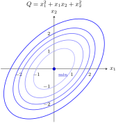
In optimization, we often want to know whether a function \(f(\mathbf{x})\) has a minimum. For a quadratic function this question reduces to a condition on its associated matrix. Geometrically, for a quadratic form in two variables, positive definiteness means the level curves \(\mathbf{x}^TA\mathbf{x} = c\) are ellipses (not hyperbolas)—the surface \(z = \mathbf{x}^TA\mathbf{x}\) is bowl-shaped and must have a minimum.

Example 7.7.15. Motivation: Does a Minimum Exist?

Consider the function
\begin{equation*} f(x_1, x_2) = x_1^2 + x_1x_2 + x_2^2 - x_1 - 3x_2. \end{equation*}
Does \(f\) have a minimum value?
Solution.
We complete the square by separating the quadratic and linear parts. The quadratic part is
\begin{equation*} Q(x_1, x_2) = x_1^2 + x_1x_2 + x_2^2 = \mathbf{x}^T\begin{bmatrix} 1 \amp 1/2 \\ 1/2 \amp 1 \end{bmatrix}\mathbf{x}. \end{equation*}
The eigenvalues of \(A = \begin{bmatrix} 1 \amp 1/2 \\ 1/2 \amp 1 \end{bmatrix}\) are \(\lambda_1 = 1/2\) and \(\lambda_2 = 3/2\text{,}\) both positive. So the quadratic part satisfies \(Q(\mathbf{x}) > 0\) for all \(\mathbf{x} \ne \mathbf{0}\text{.}\) This ensures that \(f\) grows without bound as \(\|\mathbf{x}\| \to \infty\text{,}\) so a minimum must exist.
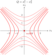
In contrast, the function \(g(x_1, x_2) = x_1^2 - x_2^2\) has quadratic part with eigenvalues \(+1\) and \(-1\text{.}\) It goes to \(+\infty\) along the \(x_1\)-axis and to \(-\infty\) along the \(x_2\)-axis, so it has neither a maximum nor a minimum.
Key observation: Whether a quadratic function has a minimum depends on whether its quadratic part is always positive—that is, whether the associated matrix is positive definite.
described in detail following the image
Contour plot of a positive definite quadratic form showing nested elliptic level curves centered at the origin.
(a) Positive definite: elliptic level curves
described in detail following the image
Contour plot of an indefinite quadratic form showing hyperbolic level curves, indicating a saddle point.
(b) Indefinite: hyperbolic level curves
Figure 7.7.16. Left: the level curves of the positive definite form \(x_1^2 + x_1 x_2 + x_2^2\) are ellipses—the surface \(z = Q(\mathbf{x})\) is bowl-shaped. Right: the level curves of the indefinite form \(x_1^2 - x_2^2\) are hyperbolas—the surface is a saddle with no minimum.

Definition 7.7.17. Positive Definite Quadratic Form and Matrix.

A quadratic form \(Q(\mathbf{x}) = \mathbf{x}^TA\mathbf{x}\) is called positive definite if
\begin{equation*} \mathbf{x}^TA\mathbf{x} > 0 \quad \text{for all } \mathbf{x} \ne \mathbf{0}. \end{equation*}
A symmetric matrix \(A\) is called positive definite if the associated quadratic form \(\mathbf{x}^TA\mathbf{x}\) is positive definite.

Example 7.7.18. Checking Positive Definiteness.

Show that the quadratic form \(f_1 = 2x_1^2 + 2x_2^2 + x_3^2 + 2x_1x_2\) is positive definite, but \(f_2 = x_1^2 + x_2^2 + x_3^2 + 2x_1x_2\) is not.
Solution.
The associated matrices are
\begin{equation*} A_1 = \begin{bmatrix} 2 \amp 1 \amp 0 \\ 1 \amp 2 \amp 0 \\ 0 \amp 0 \amp 1 \end{bmatrix}, \qquad A_2 = \begin{bmatrix} 1 \amp 1 \amp 0 \\ 1 \amp 1 \amp 0 \\ 0 \amp 0 \amp 1 \end{bmatrix}. \end{equation*}
The eigenvalues of \(A_1\) are \(1, 1, 3\)—all positive—so \(f_1\) is positive definite.
The eigenvalues of \(A_2\) are \(0, 1, 2\text{.}\) Since \(\lambda = 0\) is an eigenvalue, there exists a nonzero vector \(\mathbf{v}\) with \(A_2\mathbf{v} = \mathbf{0}\text{,}\) so \(\mathbf{v}^TA_2\mathbf{v} = 0\text{.}\) Therefore \(f_2\) is not positive definite.
Concretely, \(\mathbf{v} = (1, -1, 0)^T\) is an eigenvector for \(\lambda = 0\text{,}\) and
\begin{equation*} f_2(1, -1, 0) = 1 + 1 + 0 + 2(1)(-1) = 0, \end{equation*}
confirming that \(f_2\) can equal zero for a nonzero input.

Proof.

By the spectral theorem (Theorem 7.3.11), \(A = PDP^T\) with \(P\) orthogonal and \(D = \operatorname{diag}(\lambda_1, \ldots, \lambda_n)\text{.}\) For any nonzero \(\mathbf{x}\text{,}\) let \(\mathbf{y} = P^T\mathbf{x} \ne \mathbf{0}\text{.}\) Then
\begin{equation*} \mathbf{x}^TA\mathbf{x} = \mathbf{y}^TD\mathbf{y} = \lambda_1 y_1^2 + \lambda_2 y_2^2 + \cdots + \lambda_n y_n^2. \end{equation*}
(\(\Leftarrow\)) If all \(\lambda_i > 0\text{,}\) then since \(\mathbf{y} \ne \mathbf{0}\text{,}\) at least one \(y_k \ne 0\text{,}\) so \(\mathbf{x}^TA\mathbf{x} > 0\text{.}\)
(\(\Rightarrow\)) If some \(\lambda_k \le 0\text{,}\) choose \(\mathbf{y} = \mathbf{e}_k\text{,}\) so \(\mathbf{x} = P\mathbf{e}_k \ne \mathbf{0}\) and \(\mathbf{x}^TA\mathbf{x} = \lambda_k \le 0\text{.}\) Hence \(A\) is not positive definite.
Computing eigenvalues can be expensive. For hand calculations, the following criterion based on determinants is often more practical.

Definition 7.7.20. Leading Principal Minors.

For an \(n \times n\) matrix \(A\text{,}\) the \(k\)-th leading principal minor is the determinant of the top-left \(k \times k\) submatrix of \(A\text{,}\) for \(k = 1, 2, \ldots, n\text{.}\)
For example, the \(3 \times 3\) matrix \(A = \begin{bmatrix} a_{11} \amp a_{12} \amp a_{13} \\ a_{21} \amp a_{22} \amp a_{23} \\ a_{31} \amp a_{32} \amp a_{33} \end{bmatrix}\) has three leading principal minors:
\begin{equation*} \Delta_1 = a_{11}, \qquad \Delta_2 = \begin{vmatrix} a_{11} \amp a_{12} \\ a_{21} \amp a_{22} \end{vmatrix}, \qquad \Delta_3 = \det(A). \end{equation*}

Example 7.7.22. Using Leading Principal Minors.

Using Sylvester’s criterion, determine whether the matrices
\begin{equation*} A_1 = \begin{bmatrix} 2 \amp 1 \amp 0 \\ 1 \amp 2 \amp 0 \\ 0 \amp 0 \amp 1 \end{bmatrix} \quad \text{and} \quad A_2 = \begin{bmatrix} 1 \amp 1 \amp 0 \\ 1 \amp 1 \amp 0 \\ 0 \amp 0 \amp 1 \end{bmatrix} \end{equation*}
are positive definite.
Solution.
For \(A_1\text{:}\)
\begin{align*} \Delta_1 \amp= 2 > 0\\ \Delta_2 \amp= \begin{vmatrix} 2 \amp 1 \\ 1 \amp 2 \end{vmatrix} = 4 - 1 = 3 > 0\\ \Delta_3 \amp= \det(A_1) = 1 \cdot (4 - 1) = 3 > 0 \end{align*}
All leading principal minors are positive, so \(A_1\) is positive definite.
For \(A_2\text{:}\)
\begin{align*} \Delta_1 \amp= 1 > 0\\ \Delta_2 \amp= \begin{vmatrix} 1 \amp 1 \\ 1 \amp 1 \end{vmatrix} = 1 - 1 = 0 \not> 0 \end{align*}
Since \(\Delta_2 = 0\text{,}\) the criterion fails already at the second step. Therefore \(A_2\) is not positive definite.