Least Squares Approximation

Section 5.5 Least Squares Approximation

Why Study Least Squares?

In many real-world applications, we encounter systems of linear equations that have no exact solution. This happens, for example, when we try to fit a line or curve through data points that don’t lie exactly on any simple curve. Rather than giving up, we seek the \"best\" approximate solution\u2014the one that minimizes the error.

🔗

The least squares method is one of the most important applications of linear algebra. It provides:\n

Linear Regression: Finding the \"best fit\" line or polynomial through data points\u2014fundamental to statistics and data science.
🔗

🔗
Data Fitting: Modeling experimental data with mathematical functions in physics, chemistry, engineering, and biology.
🔗

🔗
Signal Processing: Approximating signals with simpler functions for compression and noise reduction.
🔗

🔗
Machine Learning: Training linear models to predict outcomes from features\u2014the foundation of many AI algorithms.
🔗

🔗

🔗

The Connection to Orthogonal Projection:

🔗

The least squares solution has a beautiful geometric interpretation: it is the orthogonal projection of the right-hand side vector onto the column space of the coefficient matrix. This connects our geometric understanding of projections with the algebraic problem of solving inconsistent systems.

🔗

Subsection 5.5.1 Motivation: The Inconsistent System Problem

Suppose we have more than two data points \((x_i, y_i)\) in the plane and we want to find a line \(y = c_0 + c_1x\) that passes through all of them. Substituting each data point into the line equation gives us a system:

🔗

\begin{align*} c_0 + c_1x_1 \amp= y_1\\ c_0 + c_1x_2 \amp= y_2\\ \amp\vdots\\ c_0 + c_1x_n \amp= y_n \end{align*}

🔗

In matrix form:

\begin{equation*} \begin{bmatrix}1 \amp x_1\\1 \amp x_2\\\vdots \amp \vdots\\1 \amp x_n\end{bmatrix}\begin{bmatrix}c_0\\c_1\end{bmatrix} = \begin{bmatrix}y_1\\y_2\\\vdots\\y_n\end{bmatrix} \end{equation*}

or simply \(A\mathbf{x} = \mathbf{b}\text{.}\)

🔗

The Problem: If \(n > 2\) (more equations than unknowns) and the points don’t lie exactly on a line, this system is inconsistent\u2014it has no exact solution.

🔗

The Solution: Find the vector \(\mathbf{x}\) that makes \(A\mathbf{x}\) as close as possible to \(\mathbf{b}\text{.}\) That is, minimize \(\|A\mathbf{x} - \mathbf{b}\|\text{.}\)

🔗

The vector \(\mathbf{x}\) that minimizes this distance is called the least squares solution.

🔗

Subsection 5.5.2 Geometric Interpretation

Let \(A\) be an \(n \times m\) matrix with \(n > m\) (more equations than unknowns). Consider the system \(A\mathbf{x} = \mathbf{b}\text{.}\)

🔗

Key Observations:

For any vector \(\mathbf{x} \in \mathbb{R}^m\text{,}\) the product \(A\mathbf{x}\) is a linear combination of the columns of \(A\text{.}\)
🔗

🔗
Let \(W = \{A\mathbf{x} \mid \mathbf{x} \in \mathbb{R}^m\}\) be the column space of \(A\text{.}\) This is a subspace of \(\mathbb{R}^n\text{.}\)
🔗

🔗
If \(\mathbf{b} \notin W\text{,}\) then the system \(A\mathbf{x} = \mathbf{b}\) has no solution.
🔗

🔗
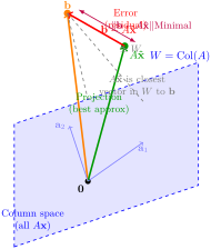
Among all vectors \(\mathbf{v} \in W\text{,}\) the distance \(d(\mathbf{b}, \mathbf{v})\) is minimized when \(\mathbf{v} = \text{proj}_W \mathbf{b}\) (the orthogonal projection of \(\mathbf{b}\) onto \(W\)).
🔗

🔗
There exists a unique \(\mathbf{\hat{x}}\) such that \(A\mathbf{\hat{x}} = \text{proj}_W \mathbf{b}\text{.}\) This \(\mathbf{\hat{x}}\) is the least squares solution.
🔗

🔗

🔗

Figure 5.5.1. Geometric interpretation of least squares: \(\mathbf{b}\) is projected onto the column space \(W\) of \(A\text{.}\) The vector \(\mathbf{b} - A\mathbf{\hat{x}}\) is orthogonal to \(W\text{.}\)
🔗

Detailed Geometric Understanding.

The least squares problem has a profound geometric interpretation that unifies projection, distance minimization, and orthogonality:

🔗

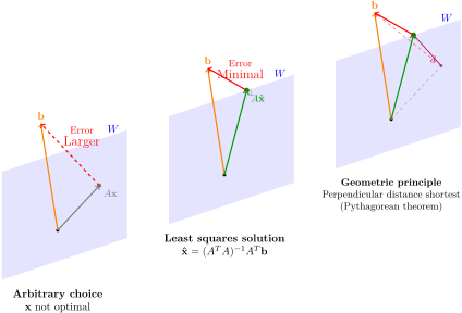
Figure 5.5.2. Why \(A\mathbf{\hat{x}}\) minimizes \(\|A\mathbf{x} - \mathbf{b}\|\text{:}\) Comparing different choices
🔗

Key geometric insights:

Projection is optimal: Among all vectors in \(W = \operatorname{Col}(A)\text{,}\) the orthogonal projection \(\text{proj}_W \mathbf{b}\) is closest to \(\mathbf{b}\text{.}\) This is \(A\mathbf{\hat{x}}\text{.}\)

🔗
Error is orthogonal: The residual \(\mathbf{b} - A\mathbf{\hat{x}}\) is perpendicular to \(W\text{.}\) This orthogonality is why we can minimize the distance—it’s the shortest path from \(\mathbf{b}\) to \(W\text{.}\)

🔗
Normal equations capture orthogonality: The condition "\(\mathbf{b} - A\mathbf{\hat{x}} \perp W\)" is algebraically expressed as \(A^T(\mathbf{b} - A\mathbf{\hat{x}}) = \mathbf{0}\text{,}\) which leads to \(A^TA\mathbf{\hat{x}} = A^T\mathbf{b}\text{.}\)

🔗
Impossible equations become possible: Even when \(A\mathbf{x} = \mathbf{b}\) has no solution (because \(\mathbf{b} \notin \operatorname{Col}(A)\)), we can always find \(\mathbf{\hat{x}}\) that makes \(A\mathbf{\hat{x}}\) as close as possible to \(\mathbf{b}\text{.}\)

🔗
Best fit interpretation: In data fitting, \(\mathbf{b}\) represents observed data, \(A\mathbf{x}\) represents model predictions. The least squares solution \(\mathbf{\hat{x}}\) gives the model parameters that best fit the data by minimizing total squared error.

🔗

🔗

Subsection 5.5.3 The Normal Equations

The key insight: \(\mathbf{b} - A\mathbf{\hat{x}}\) must be orthogonal to every vector in the column space \(W\) of \(A\text{.}\)

🔗

In particular, \(\mathbf{b} - A\mathbf{\hat{x}}\) is orthogonal to each column of \(A\text{.}\) This can be written compactly as:

\begin{equation*} A^T(\mathbf{b} - A\mathbf{\hat{x}}) = \mathbf{0} \end{equation*}

🔗

Expanding:

\begin{equation*} A^T\mathbf{b} - A^TA\mathbf{\hat{x}} = \mathbf{0} \end{equation*}

🔗

Therefore:

\begin{equation*} A^TA\mathbf{\hat{x}} = A^T\mathbf{b} \end{equation*}

🔗

Normal Equations for Least Squares.

If \(A\) is an \(n \times m\) matrix and \(\mathbf{b} \in \mathbb{R}^n\text{,}\) then the least squares solution \(\mathbf{\hat{x}}\) to the system \(A\mathbf{x} = \mathbf{b}\) satisfies the normal equations:

\begin{equation*} A^TA\mathbf{\hat{x}} = A^T\mathbf{b} \end{equation*}

🔗

If the columns of \(A\) are linearly independent, then \(A^TA\) is invertible and the unique least squares solution is:

\begin{equation*} \mathbf{\hat{x}} = (A^TA)^{-1}A^T\mathbf{b} \end{equation*}

🔗

Why This Works:

🔗

The orthogonal projection of \(\mathbf{b}\) onto \(W\) is \(\text{proj}_W \mathbf{b} = A\mathbf{\hat{x}}\text{.}\)

🔗
The error vector \(\mathbf{b} - A\mathbf{\hat{x}}\) is orthogonal to \(W\text{.}\)

🔗
This error is orthogonal to every column of \(A\text{,}\) which gives \(A^T(\mathbf{b} - A\mathbf{\hat{x}}) = \mathbf{0}\text{.}\)

🔗
Solving this equation yields the normal equations.

🔗

🔗

Subsection 5.5.4 Examples and Applications

Example 5.5.3. Solving a Simple Least Squares Problem.

Find the least squares solution of the system

\begin{equation*} \begin{bmatrix}1 \amp 1\\1 \amp 2\\1 \amp 3\end{bmatrix}\begin{bmatrix}c_0\\c_1\end{bmatrix} = \begin{bmatrix}0\\1\\3\end{bmatrix} \end{equation*}

🔗

Solution.

Here \(A = \begin{bmatrix}1 \amp 1\\1 \amp 2\\1 \amp 3\end{bmatrix}\) and \(\mathbf{b} = \begin{bmatrix}0\\1\\3\end{bmatrix}\text{.}\)

🔗

First, compute \(A^TA\text{:}\)

\begin{equation*} A^TA = \begin{bmatrix}1 \amp 1 \amp 1\\1 \amp 2 \amp 3\end{bmatrix}\begin{bmatrix}1 \amp 1\\1 \amp 2\\1 \amp 3\end{bmatrix} = \begin{bmatrix}3 \amp 6\\6 \amp 14\end{bmatrix} \end{equation*}

🔗

Next, compute \(A^T\mathbf{b}\text{:}\)

\begin{equation*} A^T\mathbf{b} = \begin{bmatrix}1 \amp 1 \amp 1\\1 \amp 2 \amp 3\end{bmatrix}\begin{bmatrix}0\\1\\3\end{bmatrix} = \begin{bmatrix}4\\11\end{bmatrix} \end{equation*}

🔗

Now solve \(A^TA\mathbf{\hat{x}} = A^T\mathbf{b}\text{:}\)

\begin{equation*} \begin{bmatrix}3 \amp 6\\6 \amp 14\end{bmatrix}\begin{bmatrix}c_0\\c_1\end{bmatrix} = \begin{bmatrix}4\\11\end{bmatrix} \end{equation*}

🔗

Row reducing the augmented matrix:

\begin{equation*} \left[\begin{array}{cc|c}3 \amp 6 \amp 4\\6 \amp 14 \amp 11\end{array}\right] \sim \left[\begin{array}{cc|c}1 \amp 0 \amp -1\\0 \amp 1 \amp 3/2\end{array}\right] \end{equation*}

🔗

Therefore, the least squares solution is \(\mathbf{\hat{x}} = \begin{bmatrix}-1\\3/2\end{bmatrix}\text{.}\)

🔗

This means the best fit line is \(y = -1 + \frac{3}{2}x\text{.}\)

🔗

Example 5.5.4. Least Squares Regression Line.

Find the least squares regression line for the points \((1,1)\text{,}\) \((2,2)\text{,}\) \((3,4)\text{,}\) \((4,4)\text{,}\) and \((5,6)\text{.}\)

🔗

Solution.

We want to find \(y = c_0 + c_1x\) that best fits these points. This gives the system:

\begin{equation*} \begin{bmatrix}1 \amp 1\\1 \amp 2\\1 \amp 3\\1 \amp 4\\1 \amp 5\end{bmatrix}\begin{bmatrix}c_0\\c_1\end{bmatrix} = \begin{bmatrix}1\\2\\4\\4\\6\end{bmatrix} \end{equation*}

🔗

Computing:

\begin{equation*} A^TA = \begin{bmatrix}5 \amp 15\\15 \amp 55\end{bmatrix}, \quad A^T\mathbf{b} = \begin{bmatrix}17\\57\end{bmatrix} \end{equation*}

🔗

Solving \(A^TA\mathbf{\hat{x}} = A^T\mathbf{b}\text{:}\)

\begin{equation*} \begin{bmatrix}5 \amp 15\\15 \amp 55\end{bmatrix}\begin{bmatrix}c_0\\c_1\end{bmatrix} = \begin{bmatrix}17\\57\end{bmatrix} \end{equation*}

🔗

This gives \(c_0 = 0.2\) and \(c_1 = 1.1\text{.}\)

🔗

Therefore, the least squares regression line is \(y = 0.2 + 1.1x\text{.}\)

🔗

Example 5.5.5. Orthogonal Projection onto Column Space.

Find the orthogonal projection of the vector \(\mathbf{b} = \begin{bmatrix}1\\1\\3\end{bmatrix}\) onto the column space of \(A = \begin{bmatrix}0 \amp 2\\3 \amp 0\\1 \amp 0\end{bmatrix}\text{.}\)

🔗

Solution.

The projection is \(\text{proj}_{\text{Col}(A)} \mathbf{b} = A\mathbf{\hat{x}}\text{,}\) where \(\mathbf{\hat{x}}\) is the least squares solution to \(A\mathbf{x} = \mathbf{b}\text{.}\)

🔗

Compute:

\begin{equation*} A^TA = \begin{bmatrix}10 \amp 0\\0 \amp 4\end{bmatrix}, \quad A^T\mathbf{b} = \begin{bmatrix}6\\2\end{bmatrix} \end{equation*}

🔗

Solving \(A^TA\mathbf{\hat{x}} = A^T\mathbf{b}\text{:}\)

\begin{equation*} \mathbf{\hat{x}} = \begin{bmatrix}3/5\\1/2\end{bmatrix} \end{equation*}

🔗

Therefore:

\begin{equation*} \text{proj}_{\text{Col}(A)} \mathbf{b} = A\mathbf{\hat{x}} = \begin{bmatrix}0 \amp 2\\3 \amp 0\\1 \amp 0\end{bmatrix}\begin{bmatrix}3/5\\1/2\end{bmatrix} = \begin{bmatrix}1\\9/5\\3/5\end{bmatrix} \end{equation*}

🔗

Subsection 5.5.5 Applications: Mathematical Modeling

Least squares problems play a fundamental role in mathematical modeling of real-world phenomena. The following examples illustrate the power and versatility of this method.

🔗

Example 5.5.6. Fitting a Quadratic Polynomial.

The table shows the world population (in billions) for six different years:

🔗

Year	1985	1990	1995	2000	2005	2010
Population	4.9	5.3	5.7	6.1	6.5	6.9

Let \(x = 5\) represent 1985. Find the least squares quadratic polynomial \(y = c_0 + c_1x + c_2x^2\) and use it to estimate the population for 2020.

🔗

Solution.

With \(x = 5, 10, 15, 20, 25, 30\) corresponding to the years, we set up:

\begin{equation*} A = \begin{bmatrix}1 \amp 5 \amp 25\\1 \amp 10 \amp 100\\1 \amp 15 \amp 225\\1 \amp 20 \amp 400\\1 \amp 25 \amp 625\\1 \amp 30 \amp 900\end{bmatrix}, \quad \mathbf{b} = \begin{bmatrix}4.9\\5.3\\5.7\\6.1\\6.5\\6.9\end{bmatrix} \end{equation*}

🔗

Solving the normal equations gives approximately:

\begin{equation*} y = 4.54 + 0.056x + 0.0006x^2 \end{equation*}

🔗

For 2020, \(x = 40\text{:}\)

\begin{equation*} y(40) = 4.54 + 0.056(40) + 0.0006(40)^2 \approx 7.94 \text{ billion} \end{equation*}

🔗

Remark 5.5.7.

Why Least Squares is Everywhere:

🔗

Statistics: Linear regression is the foundation of statistical modeling. The least squares line through data minimizes the sum of squared residuals, which has optimal statistical properties under certain assumptions.
🔗

🔗
Machine Learning: Training linear models, computing principal components (PCA), and regularized regression (Ridge, Lasso) all rely on least squares methods.
🔗

🔗
Engineering: System identification, control theory, and signal processing extensively use least squares for parameter estimation and filtering.
🔗

🔗
Computer Graphics: Fitting curves and surfaces to 3D scan data uses least squares approximation.
🔗

🔗

🔗

Exercises 5.5.6 Exercises

1.

Find the least squares solution to the system:

\begin{equation*} \begin{bmatrix}1 \amp 0\\1 \amp 1\\1 \amp 2\end{bmatrix}\begin{bmatrix}c_0\\c_1\end{bmatrix} = \begin{bmatrix}1\\2\\4\end{bmatrix} \end{equation*}

🔗

2.

Find the least squares regression line for the data points \((0,1)\text{,}\) \((1,3)\text{,}\) \((2,4)\text{,}\) \((3,5)\text{.}\)

🔗

3.

Let \(A = \begin{bmatrix}1 \amp 1\\2 \amp -1\\1 \amp 0\end{bmatrix}\) and \(\mathbf{b} = \begin{bmatrix}2\\1\\2\end{bmatrix}\text{.}\) Find the orthogonal projection of \(\mathbf{b}\) onto the column space of \(A\text{.}\)

🔗

Prev Top Next