Section 5.3 Gram-Schmidt Process

Why Do We Need the Gram-Schmidt Process?
We’ve seen that orthogonal and orthonormal bases make computations much simpler\u2014projections, coordinates, and decompositions all have clean formulas. But how do we obtain such bases in practice?
The Problem: Given an arbitrary basis \(\{\mathbf{v}_1, \mathbf{v}_2, \ldots, \mathbf{v}_n\}\) for a subspace (or vector space), find an orthonormal basis for the same space.
The Solution: The Gram-Schmidt Process is an algorithm that systematically converts any basis into an orthonormal basis. It works by processing vectors one at a time, removing components that are not orthogonal to the vectors already processed.
Why This Is Important:
  • QR Factorization: The Gram-Schmidt process underlies the QR factorization \(A = QR\text{,}\) where \(Q\) has orthonormal columns and \(R\) is upper triangular. This is essential for solving least squares problems numerically.
  • Numerical Stability: Many algorithms work better with orthonormal bases because they avoid numerical errors from nearly parallel vectors.
  • Function Spaces: Gram-Schmidt can create orthogonal polynomial bases (Legendre, Chebyshev), orthogonal trigonometric functions (Fourier), and more.
  • Signal Processing: Orthogonal wavelets and filter banks for compression and analysis are constructed using Gram-Schmidt-like procedures.
The Geometric Idea:
Starting with \(\mathbf{v}_1\text{,}\) we keep it (after normalizing). For \(\mathbf{v}_2\text{,}\) we subtract its projection onto \(\mathbf{v}_1\) to make it orthogonal. For \(\mathbf{v}_3\text{,}\) we subtract its projections onto both \(\mathbf{v}_1\) and \(\mathbf{v}_2\text{.}\) Continuing this way, we build up an orthogonal set that spans the same spaces as the original vectors.

Subsection 5.3.1 The Gram-Schmidt Algorithm

The Gram-Schmidt Process turns a basis of \(\mathbb{R}^{n}\) (or any inner product space) into an orthonormal basis.
Here are the procedures:

Gram-Schmidt Process.

Let \(B=\left\{\mathbf{v}_{1}, \mathbf{v}_{2}, \ldots, \mathbf{v}_{m}\right\}\) be a basis of a subspace \(W\) of \(\mathbb{R}^{n}\text{.}\)
Step 1: Create an Orthogonal Basis
  1. Let \(B^{\prime}=\left\{\mathbf{w}_{1}, \mathbf{w}_{2}, \ldots, \mathbf{w}_{m}\right\}\text{,}\) where
    \begin{align*} \mathbf{w}_1\amp=\mathbf{v}_1 \\ \mathbf{w}_2\amp=\mathbf{v}_2-\frac{\mathbf{v}_2\cdot \mathbf{w}_1}{\mathbf{w}_1\cdot \mathbf{w}_1}~\mathbf{w}_1 \\ \mathbf{w}_3\amp=\mathbf{v}_3-\frac{\mathbf{v}_3\cdot \mathbf{w}_1}{\mathbf{w}_1\cdot \mathbf{w}_1}~\mathbf{w}_1-\frac{\mathbf{v}_3\cdot \mathbf{w}_2}{\mathbf{w}_2\cdot \mathbf{w}_2}~\mathbf{w}_2 \\ \amp\vdots\\ \mathbf{w}_m\amp=\mathbf{v}_m-\frac{\mathbf{v}_m\cdot \mathbf{w}_1}{\mathbf{w}_1\cdot \mathbf{w}_1}~\mathbf{w}_1-\frac{\mathbf{v}_m\cdot \mathbf{w}_2}{\mathbf{w}_2\cdot \mathbf{w}_2}~\mathbf{w}_2-\ldots-\frac{\mathbf{v}_m\cdot \mathbf{w}_{m-1}}{\mathbf{w}_{m-1}\cdot \mathbf{w}_{m-1}}~\mathbf{w}_{m-1} \end{align*}
    Then \(B'\) is an orthogonal basis of \(W\text{.}\)
    Interpretation: Each \(\mathbf{w}_k\) is obtained by taking \(\mathbf{v}_k\) and subtracting off its components in the directions of all previous \(\mathbf{w}_j\)’s. This leaves only the part of \(\mathbf{v}_k\) that is orthogonal to the span of \(\{\mathbf{w}_1, \ldots, \mathbf{w}_{k-1}\}\text{.}\)
Step 2: Normalize to Create Orthonormal Basis
  1. Let \(\mathbf{u}_{i}=\frac{\mathbf{w}_{i}}{\left\|\mathbf{w}_{i}\right\|}\) for each \(i\text{.}\) Then \(B^{\prime \prime}=\left\{\mathbf{u}_{1}, \mathbf{u}_{2}, \ldots, \mathbf{u}_{m}\right\}\) is an orthonormal basis for \(W\text{.}\)
    Also, for \(k=1,2, \ldots, m\text{,}\)
    \begin{equation*} \operatorname{span}\left\{\mathbf{v}_{1}, \mathbf{v}_{2}, \ldots, \mathbf{v}_{k}\right\}=\operatorname{span}\left\{\mathbf{w}_{1}, \mathbf{w}_{2}, \ldots, \mathbf{w}_{k}\right\}=\operatorname{span}\left\{\mathbf{u}_{1}, \mathbf{u}_{2}, \ldots, \mathbf{u}_{k}\right\} \end{equation*}
    Interpretation: Dividing each orthogonal vector by its length converts it to a unit vector, giving an orthonormal basis.

Remark 5.3.1.

Key Properties of Gram-Schmidt:
  1. The spans are preserved at each step: \(\operatorname{span}\{\mathbf{v}_1, \ldots, \mathbf{v}_k\} = \operatorname{span}\{\mathbf{u}_1, \ldots, \mathbf{u}_k\}\text{.}\)
  2. The process is constructive: it gives an explicit algorithm, not just an existence proof.
  3. It works in any inner product space, not just \(\mathbb{R}^n\)\u2014we just replace dot products with inner products.
  4. The resulting orthonormal basis depends on the order of the original vectors.

Geometric Visualization of Gram-Schmidt Process.

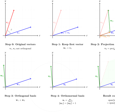
The Gram-Schmidt process has a beautiful geometric interpretation: at each step, we project out the "old" components and keep only the "new" orthogonal component. Let’s visualize this step-by-step in \(\mathbb{R}^2\text{.}\)
Figure 5.3.2. Gram-Schmidt Process in \(\mathbb{R}^2\text{:}\) Converting two non-orthogonal vectors to orthogonal vectors
The key geometric steps are:
  1. Keep \(\mathbf{v}_1\text{:}\) \(\mathbf{w}_1 = \mathbf{v}_1\) (nothing to orthogonalize against yet)
  2. Decompose \(\mathbf{v}_2\text{:}\) Split \(\mathbf{v}_2\) into two parts:
    • Component parallel to \(\mathbf{w}_1\text{:}\) \(\text{proj}_{\mathbf{w}_1}\mathbf{v}_2 = \frac{\mathbf{v}_2 \cdot \mathbf{w}_1}{\mathbf{w}_1 \cdot \mathbf{w}_1}\mathbf{w}_1\)
    • Component perpendicular to \(\mathbf{w}_1\text{:}\) \(\mathbf{w}_2 = \mathbf{v}_2 - \text{proj}_{\mathbf{w}_1}\mathbf{v}_2\)
  3. Orthogonal basis: Now \(\{\mathbf{w}_1, \mathbf{w}_2\}\) are orthogonal: \(\mathbf{w}_1 \perp \mathbf{w}_2\)
  4. Normalize: Convert to unit vectors: \(\mathbf{u}_1 = \frac{\mathbf{w}_1}{\|\mathbf{w}_1\|}\text{,}\) \(\mathbf{u}_2 = \frac{\mathbf{w}_2}{\|\mathbf{w}_2\|}\)
  5. Same span: The new basis spans the same space as the original vectors
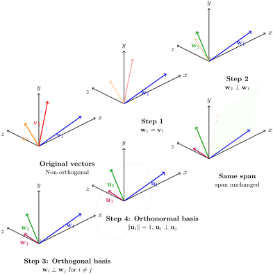
Figure 5.3.3. Gram-Schmidt Process in \(\mathbb{R}^3\text{:}\) Building an orthonormal basis step by step
For three vectors in \(\mathbb{R}^3\text{,}\) the process extends naturally:
  • Step 1: \(\mathbf{w}_1 = \mathbf{v}_1\)
  • Step 2: Make \(\mathbf{w}_2\) orthogonal to \(\mathbf{w}_1\) by removing \(\mathbf{v}_2\)’s component along \(\mathbf{w}_1\)
  • Step 3: Make \(\mathbf{w}_3\) orthogonal to both \(\mathbf{w}_1\) and \(\mathbf{w}_2\) by removing \(\mathbf{v}_3\)’s components along both
  • Step 4: Normalize all three vectors to unit length
Insight 5.3.4. The Geometric Essence of Gram-Schmidt.
  • Sequential orthogonalization: We process vectors one at a time, ensuring each new vector is orthogonal to all previous ones.
  • Projection removal: At each step, we subtract off the "parallel" components (projections) to isolate the "perpendicular" component that adds a new orthogonal direction.
  • Span preservation: At every step \(k\text{,}\) we have \(\operatorname{span}\{\mathbf{v}_1, \ldots, \mathbf{v}_k\} = \operatorname{span}\{\mathbf{w}_1, \ldots, \mathbf{w}_k\} = \operatorname{span}\{\mathbf{u}_1, \ldots, \mathbf{u}_k\}\text{.}\) The vectors span the same nested sequence of subspaces.
  • Why it works: If \(\{\mathbf{v}_1, \ldots, \mathbf{v}_n\}\) are linearly independent, each \(\mathbf{v}_k\) has a non-zero component orthogonal to \(\operatorname{span}\{\mathbf{v}_1, \ldots, \mathbf{v}_{k-1}\}\text{.}\) That component becomes \(\mathbf{w}_k\text{.}\)
  • Order matters: Different orderings of the original vectors produce different orthonormal bases (though they span the same space).

Subsection 5.3.2 Examples of Gram-Schmidt Process

Example 5.3.5. Orthonormalizing a Basis in \(\mathbb{R}^4\).

Let \(S=\{(1,2,-1,0),(2,2,0,1),(1,1,-1,0)\}\) and \(W=\operatorname{span}(S)\text{.}\) Find an orthonormal basis of \(W\) using the Gram-Schmidt process.
Computational Approach: Use Sage or Python to perform the Gram-Schmidt calculations:

Example 5.3.6.

Let \(S=\{(1,2,-1,0),(2,2,0,1),(1,1,-1,1)\}\) and \(W=\operatorname{span}(S)\text{.}\) Find a orthonormal basis of \(W\text{.}\)