Vector Space \mathbb{R}^n

Section 4.1 Vector Space \(\mathbb{R}^n\)

We begin our study of vector spaces with the most fundamental and concrete example: the vector space \(\mathbb{R}^n\text{.}\) This serves as a prototype for all vector spaces, providing a solid foundation for understanding abstract vector spaces that we will encounter later. By thoroughly studying \(\mathbb{R}^n\text{,}\) we develop intuition and computational skills that will transfer to more general settings.

🔗

Why Study \(\mathbb{R}^n\) First?

🔗

Concrete and Visual: Vectors in \(\mathbb{R}^n\) are simply column vectors with \(n\) real number entries. We can visualize \(\mathbb{R}^2\) and \(\mathbb{R}^3\) geometrically, making abstract concepts like linear independence and span more intuitive.
🔗

🔗
Computational Foundation: All fundamental concepts (linear combinations, linear independence, span, basis, dimension) can be understood and computed explicitly in \(\mathbb{R}^n\) using matrices and determinants. These computational techniques are essential for applications.
🔗

🔗
Prototype for Abstraction: Every concept we learn in \(\mathbb{R}^n\) generalizes naturally to abstract vector spaces. By mastering these ideas in a concrete setting first, we build a strong foundation for understanding polynomials, matrices, and functions as vectors.
🔗

🔗
Universal Through Coordinate Vectors: As we will see later, every finite-dimensional vector space is essentially "the same" as some \(\mathbb{R}^n\) through coordinate representations. Understanding \(\mathbb{R}^n\) thoroughly means understanding all finite-dimensional vector spaces.
🔗

🔗

🔗

In this section, we study the set

🔗

\begin{equation*} \mathbb{R}^n=\left\{\left[ \begin{array}{c} x_1 \\ x_2 \\ \vdots \\ x_n \\ \end{array} \right]\middle| x_i\in \mathbb{R} \right\} \end{equation*}

🔗

equipped with two operations:

🔗

Vector Addition:

🔗

\begin{equation*} \left[ \begin{array}{c} x_1 \\ x_2 \\ \vdots \\ x_n \\ \end{array} \right]+\left[ \begin{array}{c} y_1 \\ y_2 \\ \vdots \\ y_n \\ \end{array} \right]=\left[ \begin{array}{c} x_1+y_1 \\ x_2+y_2 \\ \vdots \\ x_n+y_n \\ \end{array} \right] \end{equation*}

🔗

Scalar Multiplication:

🔗

\begin{equation*} c\left[ \begin{array}{c} x_1 \\ x_2 \\ \vdots \\ x_n \\ \end{array} \right]=\left[ \begin{array}{c} cx_1 \\ cx_2 \\ \vdots \\ cx_n \\ \end{array} \right] \end{equation*}

🔗

These operations satisfy all the properties needed to make \(\mathbb{R}^n\) a vector space. Let us now explore the key concepts that describe the structure of this space.

🔗

Subsection 4.1.1 Span

Exploration 4.1.1. Motivation: Mixing Colors of Light.

A screen displays color by mixing three primary colors of light: Red, Green, and Blue (RGB). Each pure primary can be represented as a vector recording how much of each primary is present:

🔗

\begin{equation*} \mathbf{r} = \begin{bmatrix}1\\0\\0\end{bmatrix}, \quad \mathbf{g} = \begin{bmatrix}0\\1\\0\end{bmatrix}, \quad \mathbf{b} = \begin{bmatrix}0\\0\\1\end{bmatrix}. \end{equation*}

🔗

Any color on the screen is produced by choosing intensities \(\alpha, \beta, \gamma \geq 0\) and forming the mixture

🔗

\begin{equation*} \text{color} = \alpha\,\mathbf{r} + \beta\,\mathbf{g} + \gamma\,\mathbf{b} = \begin{bmatrix}\alpha\\\beta\\\gamma\end{bmatrix}. \end{equation*}

🔗

For example:

Yellow light: \(1\cdot\mathbf{r}+1\cdot\mathbf{g}+0\cdot\mathbf{b} = \begin{bmatrix}1\\1\\0\end{bmatrix}\)
🔗

🔗
Cyan light: \(0\cdot\mathbf{r}+1\cdot\mathbf{g}+1\cdot\mathbf{b} = \begin{bmatrix}0\\1\\1\end{bmatrix}\)
🔗

🔗
White light: \(1\cdot\mathbf{r}+1\cdot\mathbf{g}+1\cdot\mathbf{b} = \begin{bmatrix}1\\1\\1\end{bmatrix}\)
🔗

🔗

The collection of all colors obtainable this way is exactly the span of \(\{\mathbf{r},\mathbf{g},\mathbf{b}\}\text{.}\)

🔗

This everyday example captures the essence of span: start with a fixed set of building blocks, and the span is every vector you can reach by scaling and adding them. The key questions then become:

Can every color be mixed? (Does the span fill all of \(\mathbb{R}^3\text{?}\))
🔗

🔗
Could we get by with fewer primaries? (Is any one of \(\mathbf{r},\mathbf{g},\mathbf{b}\) a mixture of the other two?)
🔗

🔗

These are precisely the questions of span and linear independence that we study in this chapter.

🔗

Definition of Span.

Let \(S=\{v_1,v_2,\ldots,v_k\}\) be a subset of a vector space \(V\text{.}\) The span of \(S\) is defined as

🔗

\begin{equation*} \operatorname{span}(S)=\{x_{1}v_{1}+x_{2}v_{2}+\ldots+x_{k}v_{k}\mid x_{i}\in \mathbb{R}\} \end{equation*}

🔗

In other words, \(\operatorname{span}(S)\) is the set of all linear combinations of the vectors in \(S\text{.}\)

🔗

Example 4.1.1.

Let \(S=\left\{\left[\begin{array}{r} 1 \\ 1 \\ \end{array}\right],\left[\begin{array}{r} 0 \\ 1 \end{array}\right]\right\}\text{.}\)

🔗

\begin{equation*} \operatorname{span}(S)=\{x_{1}v_{1}+x_{2}v_{2}|x_{i}\in \mathbb{R}\}=\mathbb{R}^{2} \end{equation*}

🔗

Geometric Interpretation: The span of \(S\) is the entire plane \(\mathbb{R}^2\text{.}\) We can visualize this as follows: any vector \(\begin{bmatrix}a\\b\end{bmatrix}\) in \(\mathbb{R}^2\) can be written as a linear combination of \(v_1\) and \(v_2\text{.}\)

🔗

To see this algebraically, we need to solve:

🔗

\begin{equation*} x_1\begin{bmatrix}1\\1\end{bmatrix} + x_2\begin{bmatrix}0\\1\end{bmatrix} = \begin{bmatrix}a\\b\end{bmatrix} \end{equation*}

🔗

This gives us the system:

\begin{align*} x_1 &= a\\ x_1 + x_2 &= b \end{align*}

🔗

From the first equation, \(x_1 = a\text{.}\) Substituting into the second equation:

🔗

\begin{equation*} a + x_2 = b \quad \Rightarrow \quad x_2 = b - a \end{equation*}

🔗

Therefore, for any vector \(\begin{bmatrix}a\\b\end{bmatrix}\) in \(\mathbb{R}^2\text{,}\) we have:

🔗

\begin{equation*} \begin{bmatrix}a\\b\end{bmatrix} = a\begin{bmatrix}1\\1\end{bmatrix} + (b-a)\begin{bmatrix}0\\1\end{bmatrix} \end{equation*}

🔗

Since every vector in \(\mathbb{R}^2\) can be expressed as a linear combination of \(v_1\) and \(v_2\text{,}\) we conclude that \(\operatorname{span}(S) = \mathbb{R}^2\text{.}\)

🔗

Activity 4.1.2.

Show that the set \(S\) below spans \(\mathbb{R}^{4}\text{.}\)

🔗

\begin{equation*} S=\{v_1,v_2,v_3,v_4\}=\left\{\left[\begin{array}{r} 1 \\ 0 \\ -1 \\ 0 \end{array}\right],\left[\begin{array}{r} 1 \\ 1 \\ 0 \\ 2 \end{array}\right],\left[\begin{array}{r} 0 \\ 3 \\ 1 \\ -2 \end{array}\right],\left[\begin{array}{r} 0 \\ 1 \\ -1 \\ 2 \end{array}\right]\right\}. \end{equation*}

🔗

That is, for any \(v=\left[\begin{array}{r} a \\ b \\ c \\ d \end{array}\right]\text{,}\) the vector equation

🔗

\begin{equation*} v = x_{1}v_{1}+x_{2}v_{2}+x_{3}v_{3}+x_{4}v_{4} \end{equation*}

🔗

is consistent(has a solution).

🔗

Activity 4.1.3.

Let

🔗

\begin{equation*} S=\{v_1,v_2,v_3,v_4\}=\left\{\left[\begin{array}{r} 1 \\ 0 \\ -1 \\ 0 \end{array}\right],\left[\begin{array}{r} 1 \\ 1 \\ 0 \\ 2 \end{array}\right],\left[\begin{array}{r} 0 \\ 3 \\ 1 \\ 2 \end{array}\right],\left[\begin{array}{r} 0 \\ 1 \\ -1 \\ -2 \end{array}\right]\right\}. \end{equation*}

🔗

Suppose that \(v=\left[\begin{array}{r} a \\ b \\ c \\ d \end{array}\right]\) is in \(\operatorname{span}(S)\text{.}\) Find a relation of \(a,b,c,d\text{.}\)

🔗

Subsection 4.1.2 Linear Combinations and Linear Independence

An important type of problem in linear algebra involves writing one vector \(\mathbf{x}\) as the sum of scalar multiples of other vectors \(\mathbf{v}_{1}, \mathbf{v}_{2}, \ldots\text{,}\) and \(\mathbf{v}_{n}\text{.}\) That is, for scalars \(c_{1}\text{,}\) \(c_{2}, \ldots, c_{n}\)

🔗

\begin{equation*} \mathbf{x}=c_{1} \mathbf{v}_{1}+c_{2} \mathbf{v}_{2}+\cdots+c_{n} \mathbf{v}_{n} \end{equation*}

🔗

The vector \(\mathbf{x}\) is called a linear combination of the vectors \(\mathbf{v}_{1}, \mathbf{v}_{2}, \ldots, \mathbf{v}_{n}\) with weight \(c_1,c_2,\ldots,c_n\text{.}\)

🔗

Linear Independent Set.

A set of vectors \(\{\mathbf{v}_1,\mathbf{v}_2,\ldots,\mathbf{v}_n\}\) is called linear independent if the linear combination

🔗

\begin{equation*} x_{1} \mathbf{v}_{1}+x_{2} \mathbf{v}_{2}+\cdots+x_{n} \mathbf{v}_{n}=\mathbf{0} \end{equation*}

🔗

has only trivial solution, that is, \(x_1=x_2=\ldots =x_n=0\) is the only solution.

🔗

Geometric Interpretation of Linear Independence.

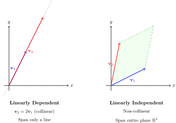
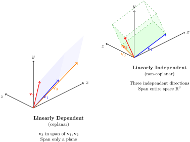
The algebraic definition of linear independence has a beautiful geometric meaning: linearly independent vectors point in fundamentally different directions, while linearly dependent vectors share directional relationships. Let’s visualize this in \(\mathbb{R}^2\) and \(\mathbb{R}^3\text{.}\)

🔗

Figure 4.1.2. Linear independence in \(\mathbb{R}^2\text{:}\) Two vectors
🔗

In \(\mathbb{R}^2\text{,}\) two vectors are:

Linearly dependent if and only if they are collinear (lie on the same line). One is a scalar multiple of the other. They span only a 1-dimensional line.

🔗
Linearly independent if and only if they are non-collinear. They point in different directions and together span the entire 2-dimensional plane \(\mathbb{R}^2\text{.}\)

🔗

🔗

Figure 4.1.3. Linear independence in \(\mathbb{R}^3\text{:}\) Three vectors
🔗

In \(\mathbb{R}^3\text{,}\) three vectors are:

Linearly dependent if and only if they are coplanar (lie on the same plane). At least one can be written as a linear combination of the others. They span at most a 2-dimensional plane.

🔗
Linearly independent if and only if they are non-coplanar. They point in three independent directions, forming a parallelepiped (3D box), and together span the entire 3-dimensional space \(\mathbb{R}^3\text{.}\)

🔗

🔗

Insight 4.1.4. The Geometric Essence of Linear Independence.

Linear independence means dimensional freedom: Each vector adds a new dimension. \(n\) linearly independent vectors in \(\mathbb{R}^n\) span the entire \(n\)-dimensional space.

🔗
Linear dependence means redundancy: At least one vector is "trapped" in the span of the others—it doesn’t add new dimensional freedom.

🔗
Testing linear independence geometrically:
- In \(\mathbb{R}^2\text{:}\) Check if vectors are collinear
  
  🔗
- In \(\mathbb{R}^3\text{:}\) Check if vectors are coplanar (equivalently: check if their scalar triple product \(\mathbf{v}_1\cdot(\mathbf{v}_2\times\mathbf{v}_3)\neq 0\))
  
  🔗
- In general: Linear independence is equivalent to the matrix \([\mathbf{v}_1\ \mathbf{v}_2\ \cdots\ \mathbf{v}_n]\) having full column rank
  
  🔗
🔗

🔗

Activity 4.1.4.

(a)

Let \(S=\{v_1,v_2,v_3,v_4\}=\left\{\left[\begin{array}{r} 1 \\ 0 \\ -1 \\ 0 \end{array}\right],\left[\begin{array}{r} 1 \\ 1 \\ 0 \\ 2 \end{array}\right],\left[\begin{array}{r} 0 \\ 3 \\ 1 \\ -2 \end{array}\right],\left[\begin{array}{r} 0 \\ 1 \\ -1 \\ 2 \end{array}\right]\right\}.\)

🔗

Show that \(S\) is linear independent.

🔗

Solution.

🔗

(b)

Let \(S=\{v_1,v_2,v_3,v_4,v_5\}=\left\{\left[\begin{array}{r} 1 \\ 0 \\ -1 \\ 0 \end{array}\right],\left[\begin{array}{r} 1 \\ 1 \\ 0 \\ 2 \end{array}\right],\left[\begin{array}{r} 0 \\ 3 \\ 1 \\ 2 \end{array}\right],\left[\begin{array}{r} 0 \\ 1 \\ -1 \\ -2 \end{array}\right], \left[\begin{array}{r} 1 \\ 1 \\ 1 \\ 1 \end{array}\right]\right\}.\)

🔗

Show that \(S\) is linear dependent.

🔗

Solution.

🔗

(c)

Write the fifth vector \(v_5\) as a linear combination of the other four vectors \(v_1, v_2,v_3\) and \(v_4\text{.}\)

🔗

Definition 4.1.5. Maximal Linear Independent Subset.

A subset \(\mathcal{M} \subseteq S\) is called a maximal linear independent subset of \(S\) if:

\(\mathcal{M}\) is linearly independent

🔗
For any vector \(\mathbf{v} \in S \setminus \mathcal{M}\text{,}\) the set \(\mathcal{M} \cup \{\mathbf{v}\}\) is linearly dependent

🔗

🔗

In other words, \(\mathcal{M}\) is a linearly independent subset that cannot be enlarged by adding any other vector from \(S\) while preserving linear independence.

🔗

Activity 4.1.5.

Find a maximal linear independent subset of the set

🔗

\begin{equation*} S=\{v_1,v_2,v_3,v_4,v_5\}=\left\{\left[\begin{array}{r} 1 \\ 0 \\ -1 \\ 0 \end{array}\right],\left[\begin{array}{r} 1 \\ 1 \\ 0 \\ 2 \end{array}\right],\left[\begin{array}{r} 0 \\ 3 \\ 1 \\ 2 \end{array}\right],\left[\begin{array}{r} 0 \\ 1 \\ -1 \\ -2 \end{array}\right], \left[\begin{array}{r} 1 \\ 1 \\ 1 \\ 1 \end{array}\right]\right\}. \end{equation*}

🔗

Insight 4.1.6. Linear Independence and Solution of Systems.

There is a profound connection between linear independence/dependence and the existence of solutions to homogeneous linear systems.

🔗

Subsection 4.1.3 Basis

Definition 4.1.7. Basis.

A set \(\mathcal{B} = \{\mathbf{v}_1, \mathbf{v}_2, \ldots, \mathbf{v}_n\}\) of vectors in \(\mathbb{R}^{n}\) is called a basis for \(\mathbb{R}^{n}\) if:

\(\mathcal{B}\) is linearly independent

🔗
\(\mathcal{B}\) spans \(\mathbb{R}^{n}\text{,}\) that is, \(\operatorname{span}(\mathcal{B}) = \mathbb{R}^{n}\)

🔗

🔗

Activity 4.1.6.

(a)

Show that the following set is a basis for \(\mathbb{R}^{2}\text{:}\) \(\left\{\begin{bmatrix}1\\3\end{bmatrix}, \begin{bmatrix}2\\4\end{bmatrix}\right\}\)

🔗

(b)

Show that the following set is a basis for \(\mathbb{R}^{3}\text{:}\) \(\left\{\begin{bmatrix}1\\1\\1\end{bmatrix}, \begin{bmatrix}1\\1\\0\end{bmatrix}, \begin{bmatrix}1\\0\\0\end{bmatrix}\right\}\)

🔗

A basis provides the most efficient way to describe a vector space: it gives us the minimum number of vectors needed to span the entire space, with no redundancy (since they are linearly independent).

🔗

Theorem 4.1.8. Basis Test via Determinant.

Let \(\mathcal{B} = \{\mathbf{v}_1, \mathbf{v}_2, \ldots, \mathbf{v}_n\}\) be a set of \(n\) vectors in \(\mathbb{R}^n\text{,}\) and let \(B\) be the \(n \times n\) matrix with columns \(\mathbf{v}_1, \mathbf{v}_2, \ldots, \mathbf{v}_n\text{.}\) Then \(\mathcal{B}\) is a basis for \(\mathbb{R}^n\) if and only if \(\det(B) \neq 0\text{.}\)

🔗

Proof.

Direction 1: If \(\mathcal{B}\) is a basis, then \(\mathcal{B}\) is linearly independent. This means the homogeneous system \(B\mathbf{x} = \mathbf{0}\) has only the trivial solution, which occurs if and only if \(\det(B) \neq 0\text{.}\)

🔗

Direction 2: If \(\det(B) \neq 0\text{,}\) then \(B\) is invertible, so the columns of \(B\) are linearly independent. Since we have \(n\) linearly independent vectors in \(\mathbb{R}^n\text{,}\) they automatically span \(\mathbb{R}^n\text{,}\) making \(\mathcal{B}\) a basis.

🔗

Example 4.1.9. Testing if a Set is a Basis.

Consider the first four vectors from activity 4.1.1:

🔗

\begin{equation*} \mathcal{B} = \left\{\mathbf{v}_1, \mathbf{v}_2, \mathbf{v}_3, \mathbf{v}_4\right\} = \left\{\begin{bmatrix}1\\0\\-1\\0\end{bmatrix}, \begin{bmatrix}1\\1\\0\\2\end{bmatrix}, \begin{bmatrix}0\\3\\1\\-2\end{bmatrix}, \begin{bmatrix}0\\1\\-1\\2\end{bmatrix}\right\} \end{equation*}

🔗

Determine whether \(\mathcal{B}\) is a basis for \(\mathbb{R}^4\text{.}\)

🔗

Solution.

To test if \(\mathcal{B}\) is a basis for \(\mathbb{R}^4\text{,}\) we form the matrix \(B\) with these vectors as columns and compute its determinant.

🔗

From the computation above, we can see that \(\det(B) \neq 0\text{,}\) which confirms that \(\mathcal{B} = \{\mathbf{v}_1, \mathbf{v}_2, \mathbf{v}_3, \mathbf{v}_4\}\) is indeed a basis for \(\mathbb{R}^4\text{.}\)

🔗

Key Insights:

The determinant test provides a quick computational method to verify if a set of vectors forms a basis.

🔗
For \(n\) vectors in \(\mathbb{R}^n\text{,}\) linear independence automatically implies spanning the entire space.

🔗
This result will be useful later when we work with coordinate vectors relative to this basis.

🔗

🔗

Activity 4.1.7.

Practice: Use the determinant test to verify whether each of the following sets forms a basis for \(\mathbb{R}^3\text{:}\)

🔗

\(\displaystyle \left\{\begin{bmatrix}1\\0\\1\end{bmatrix}, \begin{bmatrix}0\\1\\1\end{bmatrix}, \begin{bmatrix}1\\1\\0\end{bmatrix}\right\}\)

🔗
\(\displaystyle \left\{\begin{bmatrix}1\\2\\3\end{bmatrix}, \begin{bmatrix}2\\4\\6\end{bmatrix}, \begin{bmatrix}1\\0\\1\end{bmatrix}\right\}\)

🔗

🔗

Theorem 4.1.10. Basis Test via span.

Let \(\mathcal{B} = \{\mathbf{v}_1, \mathbf{v}_2, \ldots, \mathbf{v}_n\}\) be a set of \(n\) vectors in \(\mathbb{R}^n\) Then \(\mathcal{B}\) is a basis for \(\mathbb{R}^n\) if and only if \(\operatorname{Span}(\mathcal{B}) = \mathbb{R}^n\text{.}\)

🔗

Prev Top Next