The definition and its matrix of a Linear Transformation

Section 6.1 The definition and its matrix of a Linear Transformation

Subsection 6.1.1 Linear Transformation

Before we define linear transformations, let us recall some basic terminology about functions.

A function (or map) \(T: V \rightarrow W\) assigns to each vector \(\mathbf{v}\in V\) a unique vector \(T(\mathbf{v})\in W\text{.}\) We call \(V\) the domain and \(W\) the codomain. For a vector \(\mathbf{v}\in V\text{,}\) the vector \(T(\mathbf{v})\) is called the image of \(\mathbf{v}\) under \(T\text{.}\) If \(T(\mathbf{v}) = \mathbf{w}\text{,}\) we say \(\mathbf{v}\) is a preimage of \(\mathbf{w}\text{.}\)

🔗

Example 6.1.1. A simple example.

Consider the map \(T:\mathbb{R}^{2}\rightarrow \mathbb{R}^{2}\) defined by

\begin{equation*} T\left(\begin{array}{c} x \\ y \end{array}\right) = \left(\begin{array}{c} 2x \\ 3y \end{array}\right). \end{equation*}

🔗

For the vector \(\mathbf{v} = \begin{pmatrix} 1 \\ 2 \end{pmatrix}\text{,}\) its image is

\begin{equation*} T(\mathbf{v}) = T\left(\begin{array}{c} 1 \\ 2 \end{array}\right) = \left(\begin{array}{c} 2 \\ 6 \end{array}\right). \end{equation*}

So \(\begin{pmatrix} 1 \\ 2 \end{pmatrix}\) is a preimage of \(\begin{pmatrix} 2 \\ 6 \end{pmatrix}\text{.}\)

🔗

Similarly, the image of \(\begin{pmatrix} 0 \\ 0 \end{pmatrix}\) is \(\begin{pmatrix} 0 \\ 0 \end{pmatrix}\text{,}\) and the image of \(\begin{pmatrix} -1 \\ 1 \end{pmatrix}\) is \(\begin{pmatrix} -2 \\ 3 \end{pmatrix}\text{.}\)

🔗

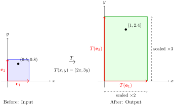
described in detail following the image — Figure 6.1.2. Geometric Effect of the Linear Transformation \(T(x,y) = (2x, 3y)\)
🔗

Geometric interpretation: This transformation performs non-uniform scaling—it stretches the x-direction by a factor of 2 and the y-direction by a factor of 3. The unit square transforms into a \(2 \times 3\) rectangle. Notice that:

The origin stays fixed: \(T(\mathbf{0}) = \mathbf{0}\)
🔗

🔗
Straight lines remain straight
🔗

🔗
Parallel lines remain parallel
🔗

🔗
The grid structure is preserved but deformed
🔗

🔗

These properties are characteristic of all linear transformations!

🔗

Definition 6.1.3. Linear Transformation.

Let \(V\) and \(W\) be finite-dimensional vector spaces. A function \(T: V \rightarrow W\) is called a linear transformation (or linear map) when the two properties below are true for all \(\mathbf{u}\) and \(\mathbf{v}\) in \(V\) and for any scalar \(c\in \mathbb{R}\text{:}\)

\begin{equation*} T(\mathbf{u}+\mathbf{v})=T(\mathbf{u})+T(\mathbf{v})\quad\text{ and } \quad T(c \mathbf{u})=c T(\mathbf{u}). \end{equation*}

🔗

The first property says \(T\) preserves addition, and the second says \(T\) preserves scalar multiplication.

🔗

Let us verify that the map in Example 6.1.1 is indeed linear. For any vectors \(\mathbf{u} = \begin{pmatrix} x_1 \\ y_1 \end{pmatrix}\) and \(\mathbf{v} = \begin{pmatrix} x_2 \\ y_2 \end{pmatrix}\text{,}\) we have

\begin{align*} T(\mathbf{u}+\mathbf{v}) \amp= T\left(\begin{array}{c} x_1+x_2 \\ y_1+y_2 \end{array}\right) = \left(\begin{array}{c} 2(x_1+x_2) \\ 3(y_1+y_2) \end{array}\right)\\ \amp= \left(\begin{array}{c} 2x_1 + 2x_2 \\ 3y_1 + 3y_2 \end{array}\right) = \left(\begin{array}{c} 2x_1 \\ 3y_1 \end{array}\right) + \left(\begin{array}{c} 2x_2 \\ 3y_2 \end{array}\right)\\ \amp= T(\mathbf{u}) + T(\mathbf{v}). \end{align*}

Similarly, for any scalar \(c\text{,}\)

\begin{equation*} T(c\mathbf{u}) = T\left(\begin{array}{c} cx_1 \\ cy_1 \end{array}\right) = \left(\begin{array}{c} 2cx_1 \\ 3cy_1 \end{array}\right) = c\left(\begin{array}{c} 2x_1 \\ 3y_1 \end{array}\right) = cT(\mathbf{u})\text{.} \end{equation*}

Therefore \(T\) is linear.

🔗

Example 6.1.4.

Show that the map \(T:\mathbb{R}^{4}\rightarrow \mathbb{R}^{4}\) defined by

\begin{equation*} T\left(\begin{array}{r} x_1 \\ x_2 \\ x_3\\ x_4 \end{array}\right)=\left(\begin{array}{r} x_1+x_2 \\ x_2+3x_3+x_4 \\ -x_1+x_3-x_4\\ 2x_2+2x_3-2x_4 \end{array}\right) \end{equation*}

is a linear transformation.

🔗

Example 6.1.5. Finding \(T(\vec{v}_1)\) and \(T(\vec{v}_2)\) from Given Information.

Let \(V\) be a vector space, and \(T: V \rightarrow V\) be a linear transformation such that

\begin{equation*} T\left(5 \vec{v}_1+3 \vec{v}_2\right)=-2 \vec{v}_1-2 \vec{v}_2 \end{equation*}

and

\begin{equation*} T\left(3 \vec{v}_1+2 \vec{v}_2\right)=2 \vec{v}_1-3 \vec{v}_2. \end{equation*}

Find:

\(\displaystyle T\left(\vec{v}_1\right)\)
🔗

🔗
\(\displaystyle T\left(\vec{v}_2\right)\)
🔗

🔗
\(\displaystyle T\left(-2 \vec{v}_1+2 \vec{v}_2\right)\)
🔗

🔗

🔗

Solution.

Key Idea: We need to express \(\vec{v}_1\) and \(\vec{v}_2\) as linear combinations of \(5\vec{v}_1+3\vec{v}_2\) and \(3\vec{v}_1+2\vec{v}_2\text{.}\) Then we can use linearity to compute \(T(\vec{v}_1)\) and \(T(\vec{v}_2)\text{.}\)

🔗

Step 1: Express \(\vec{v}_1\) as a linear combination.

🔗

We want to find constants \(a\) and \(b\) such that

\begin{equation*} \vec{v}_1 = a\left(5\vec{v}_1+3\vec{v}_2\right) + b\left(3\vec{v}_1+2\vec{v}_2\right). \end{equation*}

Expanding the right side:

\begin{equation*} \vec{v}_1 = (5a+3b)\vec{v}_1 + (3a+2b)\vec{v}_2. \end{equation*}

Comparing coefficients, we get the system:

\begin{align*} 5a + 3b \amp= 1\\ 3a + 2b \amp= 0 \end{align*}

🔗

From the second equation: \(b = -\frac{3a}{2}\text{.}\) Substituting into the first equation:

\begin{align*} 5a + 3\left(-\frac{3a}{2}\right) \amp= 1\\ 5a - \frac{9a}{2} \amp= 1\\ \frac{10a - 9a}{2} \amp= 1\\ \frac{a}{2} \amp= 1\\ a \amp= 2 \end{align*}

Therefore, \(b = -\frac{3(2)}{2} = -3\text{.}\)

🔗

We can verify: \(5(2) + 3(-3) = 10 - 9 = 1\) ✓ and \(3(2) + 2(-3) = 6 - 6 = 0\) ✓.

🔗

Thus:

\begin{equation*} \vec{v}_1 = 2\left(5\vec{v}_1+3\vec{v}_2\right) - 3\left(3\vec{v}_1+2\vec{v}_2\right). \end{equation*}

🔗

Step 2: Express \(\vec{v}_2\) as a linear combination.

🔗

Similarly, we want to find constants \(c\) and \(d\) such that

\begin{equation*} \vec{v}_2 = c\left(5\vec{v}_1+3\vec{v}_2\right) + d\left(3\vec{v}_1+2\vec{v}_2\right). \end{equation*}

This gives us:

\begin{align*} 5c + 3d \amp= 0\\ 3c + 2d \amp= 1 \end{align*}

🔗

From the first equation: \(d = -\frac{5c}{3}\text{.}\) Substituting into the second:

\begin{align*} 3c + 2\left(-\frac{5c}{3}\right) \amp= 1\\ 3c - \frac{10c}{3} \amp= 1\\ \frac{9c - 10c}{3} \amp= 1\\ -\frac{c}{3} \amp= 1\\ c \amp= -3 \end{align*}

Therefore, \(d = -\frac{5(-3)}{3} = 5\text{.}\)

🔗

We can verify: \(5(-3) + 3(5) = -15 + 15 = 0\) ✓ and \(3(-3) + 2(5) = -9 + 10 = 1\) ✓.

🔗

Thus:

\begin{equation*} \vec{v}_2 = -3\left(5\vec{v}_1+3\vec{v}_2\right) + 5\left(3\vec{v}_1+2\vec{v}_2\right). \end{equation*}

🔗

Step 3: Compute \(T(\vec{v}_1)\text{.}\)

🔗

Using linearity of \(T\text{:}\)

\begin{align*} T(\vec{v}_1) \amp= T\left(2\left(5\vec{v}_1+3\vec{v}_2\right) - 3\left(3\vec{v}_1+2\vec{v}_2\right)\right)\\ \amp= 2T\left(5\vec{v}_1+3\vec{v}_2\right) - 3T\left(3\vec{v}_1+2\vec{v}_2\right)\\ \amp= 2\left(-2\vec{v}_1-2\vec{v}_2\right) - 3\left(2\vec{v}_1-3\vec{v}_2\right)\\ \amp= -4\vec{v}_1 - 4\vec{v}_2 - 6\vec{v}_1 + 9\vec{v}_2\\ \amp= -10\vec{v}_1 + 5\vec{v}_2 \end{align*}

🔗

Step 4: Compute \(T(\vec{v}_2)\text{.}\)

🔗

\begin{align*} T(\vec{v}_2) \amp= T\left(-3\left(5\vec{v}_1+3\vec{v}_2\right) + 5\left(3\vec{v}_1+2\vec{v}_2\right)\right)\\ \amp= -3T\left(5\vec{v}_1+3\vec{v}_2\right) + 5T\left(3\vec{v}_1+2\vec{v}_2\right)\\ \amp= -3\left(-2\vec{v}_1-2\vec{v}_2\right) + 5\left(2\vec{v}_1-3\vec{v}_2\right)\\ \amp= 6\vec{v}_1 + 6\vec{v}_2 + 10\vec{v}_1 - 15\vec{v}_2\\ \amp= 16\vec{v}_1 - 9\vec{v}_2 \end{align*}

🔗

Step 5: Compute \(T(-2\vec{v}_1+2\vec{v}_2)\text{.}\)

🔗

\begin{align*} T\left(-2\vec{v}_1+2\vec{v}_2\right) \amp= -2T(\vec{v}_1) + 2T(\vec{v}_2)\\ \amp= -2\left(-10\vec{v}_1 + 5\vec{v}_2\right) + 2\left(16\vec{v}_1 - 9\vec{v}_2\right)\\ \amp= 20\vec{v}_1 - 10\vec{v}_2 + 32\vec{v}_1 - 18\vec{v}_2\\ \amp= 52\vec{v}_1 - 28\vec{v}_2 \end{align*}

🔗

Final Answers:

\begin{align*} T(\vec{v}_1) \amp= -10\vec{v}_1 + 5\vec{v}_2\\ T(\vec{v}_2) \amp= 16\vec{v}_1 - 9\vec{v}_2\\ T(-2\vec{v}_1+2\vec{v}_2) \amp= 52\vec{v}_1 - 28\vec{v}_2 \end{align*}

🔗

Theorem 6.1.6.

Let \(T\) be a linear transformation from \(V\) to \(W\text{.}\) Then

\begin{equation*} T(\mathbf{0}_V)=\mathbf{0}_W. \end{equation*}

🔗

Proof.

Since \(T\) preserves scalar multiplication, we have:

\begin{align*} T(\mathbf{0}_V) \amp= T(0 \cdot \mathbf{0}_V)\\ \amp= 0 \cdot T(\mathbf{0}_V)\\ \amp= \mathbf{0}_W \end{align*}

🔗

Thus it is a necessary condition for \(T\) to be a linear transformation.

🔗

Example 6.1.7.

Is the map \(T:\mathbb{R}^{4}\rightarrow \mathbb{R}^{4}\) linear? where \(T\) is defined by

\begin{equation*} T\left(\begin{array}{r} x_1 \\ x_2 \\ x_3\\ x_4 \end{array}\right)=\left(\begin{array}{r} x_1+x_2+2\\ x_2+3x_3+x_4 \\ -x_1+x_3-x_4\\ 2x_2+2x_3-2x_4 \end{array}\right) \end{equation*}

🔗

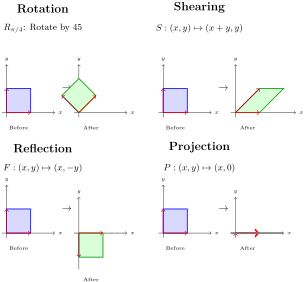
Example 6.1.8. Common Types of Linear Transformations in \(\mathbb{R}^2\).

Here are some fundamental geometric transformations that are all linear. Understanding these basic building blocks helps us understand more complex transformations.

🔗

Key observations about these transformations:

Rotation preserves lengths and angles. It’s an isometry (distance-preserving).
🔗

🔗
Shearing preserves areas but distorts shapes. Horizontal lines stay horizontal.
🔗

🔗
Reflection flips space across a line (here, the x-axis). Also an isometry.
🔗

🔗
Projection collapses a dimension. The y-coordinate is "lost" in the transformation.
🔗

🔗

🔗

All of these transformations share the fundamental properties that define linearity: they preserve vector addition and scalar multiplication, they map lines to lines, and they keep the origin fixed. Later, we’ll see that each can be represented by a simple matrix!

🔗

Example 6.1.10.

Show that the map \(T:P_{2}(x)\rightarrow P_{2}(x)\) defined by

\begin{equation*} T\left(f(x)\right)=(x-2)f'(x)+f(x) \end{equation*}

is a linear transformation.

🔗

🔗
Compute all polynomials \(f(x)=x^{2}+bx+c\) such that \(T(f(x))=3f(x)\)
🔗

🔗
Suppose that \(f(x)=a_nx^n+a_{n-1}x^{n-1}+\ldots + a_1x+a_0\text{,}\) where \(a_n \neq 0\text{.}\) \(a_n\) is called the leading coefficient, and the polynomial is called monic if \(a_n=1\text{.}\) Challenge Question: Find all possible values \(k\) and monic polynomials \(f(x)\) such that \(T(f(x))=kf(x)\)
🔗

🔗

🔗

Linear transformations are the simplest kind of maps.

🔗

In general, a function \(f:V\rightarrow W\) between vector spaces can be arbitrarily complicated — to fully understand it, we would need to know \(f(v)\) for every vector \(v\in V\text{,}\) which is often impossible since \(V\) has infinitely many vectors. But linear transformations are special: they are completely determined by what they do to a basis.

🔗

This is what makes linear transformations so tractable. If \(\{\mathbf{v}_1,\mathbf{v}_2,\ldots,\mathbf{v}_n\}\) is a basis of \(V\text{,}\) then once we know \(T(\mathbf{v}_1), T(\mathbf{v}_2),\ldots, T(\mathbf{v}_n)\) — just \(n\) vectors — we can compute \(T(\mathbf{v})\) for any vector \(\mathbf{v}\in V\text{.}\) This is because any \(\mathbf{v}\) can be written as a linear combination of the basis vectors, and linearity tells us exactly how \(T\) acts on linear combinations.

🔗

The following theorem makes this precise.

🔗

Theorem 6.1.11.

Let \(T\) be a linear transformation from \(V\) to \(W\text{,}\) and \(\{\mathbf{v}_1,\mathbf{v}_2,\ldots,\mathbf{v}_n\}\) be a basis of \(V\text{.}\) Then \(T\) is totally determined the image of \(\{\mathbf{v}_1,\mathbf{v}_2,\ldots,\mathbf{v}_n\}\text{.}\) That is, if knowing \(T(\mathbf{v}_1),T(\mathbf{v}_2),\ldots,T(\mathbf{v}_n)\text{,}\) then we know \(T(v)\) for any vector \(v\in V\text{.}\)

🔗

Proof.

\(\forall v\in V\text{,}\) since \(\{\mathbf{v}_1,\mathbf{v}_2,\ldots,\mathbf{v}_k\}\) is a basis of \(V\text{,}\)

\begin{equation*} v = x_{1}\mathbf{v}_{1}+x_{2}\mathbf{v}_{2}+\ldots+x_{n}\mathbf{v}_{n} \end{equation*}

Then we have

\begin{align*} T(v)=\amp T(x_{1}\mathbf{v}_{1}+x_{2}\mathbf{v}_{2}+\ldots+x_{n}\mathbf{v}_{n})\\ =\amp T(x_{1}\mathbf{v}_{1})+T(x_{2}\mathbf{v}_{2})+\ldots+T(x_{n}\mathbf{v}_{n})\\ =\amp x_{1}T(\mathbf{v}_{1})+x_{2}T(\mathbf{v}_{2})+\ldots+x_{n}T(\mathbf{v}_{n}) \end{align*}

🔗

Example 6.1.12. Computing Transformation Using Linearity.

If \(T: \mathbb{R}^3 \rightarrow \mathbb{R}^3\) is a linear transformation such that

\begin{equation*} T\left(\begin{bmatrix}1\\0\\0\end{bmatrix}\right)=\begin{bmatrix}0\\1\\4\end{bmatrix}, \quad T\left(\begin{bmatrix}0\\1\\0\end{bmatrix}\right)=\begin{bmatrix}2\\-2\\-3\end{bmatrix}, \quad T\left(\begin{bmatrix}0\\0\\1\end{bmatrix}\right)=\begin{bmatrix}-4\\4\\-3\end{bmatrix}, \end{equation*}

then find \(T\left(\begin{bmatrix}-3\\-4\\1\end{bmatrix}\right)\text{.}\)

🔗

Solution.

Since \(T\) is linear and we know the images of the standard basis vectors, we can use linearity to compute \(T\) for any vector in \(\mathbb{R}^3\text{.}\)

🔗

First, express the input vector as a linear combination of the standard basis:

\begin{equation*} \begin{bmatrix}-3\\-4\\1\end{bmatrix} = -3\begin{bmatrix}1\\0\\0\end{bmatrix} - 4\begin{bmatrix}0\\1\\0\end{bmatrix} + 1\begin{bmatrix}0\\0\\1\end{bmatrix}. \end{equation*}

🔗

By the linearity of \(T\text{:}\)

\begin{align*} T\left(\begin{bmatrix}-3\\-4\\1\end{bmatrix}\right) \amp= T\left(-3\begin{bmatrix}1\\0\\0\end{bmatrix} - 4\begin{bmatrix}0\\1\\0\end{bmatrix} + 1\begin{bmatrix}0\\0\\1\end{bmatrix}\right)\\ \amp= -3T\left(\begin{bmatrix}1\\0\\0\end{bmatrix}\right) - 4T\left(\begin{bmatrix}0\\1\\0\end{bmatrix}\right) + T\left(\begin{bmatrix}0\\0\\1\end{bmatrix}\right)\\ \amp= -3\begin{bmatrix}0\\1\\4\end{bmatrix} - 4\begin{bmatrix}2\\-2\\-3\end{bmatrix} + \begin{bmatrix}-4\\4\\-3\end{bmatrix}\\ \amp= \begin{bmatrix}0\\-3\\-12\end{bmatrix} + \begin{bmatrix}-8\\8\\12\end{bmatrix} + \begin{bmatrix}-4\\4\\-3\end{bmatrix}\\ \amp= \begin{bmatrix}0-8-4\\-3+8+4\\-12+12-3\end{bmatrix}\\ \amp= \begin{bmatrix}-12\\9\\-3\end{bmatrix} \end{align*}

🔗

Answer: \(T\left(\begin{bmatrix}-3\\-4\\1\end{bmatrix}\right) = \begin{bmatrix}-12\\9\\-3\end{bmatrix}\text{.}\)

🔗

Example 6.1.13. Linear Transformation on Polynomial Space.

Let \(T: P_3 \rightarrow P_3\) be the linear transformation satisfying

\begin{equation*} T(1)=2 x^2+8, \quad T(x)=-3 x-8, \quad T\left(x^2\right)=-2 x^2-x-7. \end{equation*}

Find the image of an arbitrary quadratic polynomial \(a x^2+b x+c\text{:}\)

\begin{equation*} T\left(a x^2+b x+c\right) = {?} \end{equation*}

🔗

Solution.

Since \(T\) is linear and we know the images of the basis vectors \(\{1, x, x^2\}\text{,}\) we can compute \(T\) for any polynomial in \(P_3\) by using linearity.

🔗

For an arbitrary quadratic polynomial \(ax^2 + bx + c\text{,}\) we apply the linearity of \(T\text{:}\)

\begin{align*} T\left(ax^2 + bx + c\right) \amp= T\left(ax^2\right) + T(bx) + T(c)\\ \amp= aT\left(x^2\right) + bT(x) + cT(1)\\ \amp= a\left(-2x^2 - x - 7\right) + b(-3x - 8) + c(2x^2 + 8)\\ \amp= -2ax^2 - ax - 7a - 3bx - 8b + 2cx^2 + 8c \end{align*}

🔗

Collecting terms by powers of \(x\text{:}\)

\begin{align*} T\left(ax^2 + bx + c\right) \amp= (-2a + 2c)x^2 + (-a - 3b)x + (-7a - 8b + 8c) \end{align*}

🔗

Answer:

\begin{equation*} T\left(ax^2 + bx + c\right) = \boxed{(-2a + 2c)x^2 + (-a - 3b)x + (-7a - 8b + 8c)} \end{equation*}

or equivalently,

\begin{equation*} T\left(ax^2 + bx + c\right) = \boxed{2(c-a)x^2 - (a + 3b)x + 8c - 8b - 7a}. \end{equation*}

🔗

In next subsection, we study the special case: \(V=\mathbb{R}^{n}\) and \(W = \mathbb{R}^{m}\text{.}\)

🔗

Subsection 6.1.2 Linear Transformation \(T:\mathbb{R}^{n}\rightarrow \mathbb{R}^{m}\)

Definition 6.1.14. Standard Matrix.

Let \(T\) be a linear transformation from \(\mathbb{R}^{n}\) to \(\mathbb{R}^{m}\text{,}\) and \(\{\mathbf{e}_1,\mathbf{e}_2,\ldots,\mathbf{e}_n\}\) be the standard basis of \(\mathbb{R}^{n}\text{.}\) Then \(\forall v\in V,\)

\begin{equation*} T(v)=Av, \end{equation*}

where \(A=\Big[T(\mathbf{e}_1)\, T(\mathbf{e}_2)\,\ldots\, T(\mathbf{e}_n)\Big]\text{.}\)

🔗

The matrix \(A\) is called the standard matrix of \(T\text{.}\)

🔗

Example: Let \(T:\mathbb{R}^{3}\rightarrow \mathbb{R}^{3}\) be a linear transformation such that

\begin{equation*} T\left(\begin{array}{r} 1 \\ 0 \\ 0 \end{array}\right)=\left(\begin{array}{r} 1 \\ 3\\ 0 \end{array}\right),T\left(\begin{array}{r} 0 \\ 1 \\ 0 \end{array}\right)=\left(\begin{array}{r} 3 \\ 1 \\ 0 \end{array}\right),T\left(\begin{array}{r} 0 \\ 0 \\ 1 \end{array}\right)=\left(\begin{array}{r} 0 \\ 0 \\ -2 \end{array}\right). \end{equation*}

Find the standard matrix \(A\text{.}\)

🔗

Exercise: Let \(T:\mathbb{R}^{3}\rightarrow \mathbb{R}^{3}\) be a linear transformation such that

\begin{equation*} T\left(\begin{array}{r} 1 \\ 0 \\ 0 \end{array}\right)=\left(\begin{array}{r} 1 \\ 3\\ 0 \end{array}\right),T\left(\begin{array}{r} 1 \\ 1 \\ 0 \end{array}\right)=\left(\begin{array}{r} 4 \\ 4 \\ 0 \end{array}\right),T\left(\begin{array}{r} 1 \\ 1 \\ 1 \end{array}\right)=\left(\begin{array}{r} 4 \\ 4 \\ -2 \end{array}\right). \end{equation*}

Find the standard matrix \(A\text{.}\)

🔗

Exercise: Find the standard matrix of the linear transformation in Example 6.1.4.

🔗

Activity 6.1.1. (Tough) Computing the Reflection Matrix for a Line.

Find the matrix \(A\) of the reflection in the line \(L\) in \(\mathbb{R}^2\) that consists of all scalar multiples of the vector \(\begin{bmatrix} 5 \\ 3 \end{bmatrix}\text{.}\)

🔗

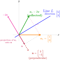
Strategy: To find the matrix \(A\text{,}\) we need to find where \(A\) sends the standard basis vectors \(\mathbf{e}_1 = \begin{bmatrix} 1 \\ 0 \end{bmatrix}\) and \(\mathbf{e}_2 = \begin{bmatrix} 0 \\ 1 \end{bmatrix}\text{.}\) The key insight is: to reflect \(\mathbf{e}_1\) across line \(L\text{,}\) we subtract twice its projection \(\mathbf{v}\) to get the reflected vector(in color Green), see the graph below for details.

🔗

(a) Step 1: Find the Perpendicular Direction.

First, we need to find a vector \(\mathbf{n}\) that is perpendicular to the line \(L\) (which has direction \(\begin{bmatrix} 5 \\ 3 \end{bmatrix}\)).

🔗

If \(\mathbf{n} = \begin{bmatrix} a \\ b \end{bmatrix}\) is perpendicular to \(\begin{bmatrix} 5 \\ 3 \end{bmatrix}\text{,}\) what equation must \(a\) and \(b\) satisfy?

🔗

Hint.

Two vectors are perpendicular if and only if their dot product is zero.

🔗

Solution.

For \(\mathbf{n} = \begin{bmatrix} a \\ b \end{bmatrix}\) to be perpendicular to \(\begin{bmatrix} 5 \\ 3 \end{bmatrix}\text{,}\) we need:

\begin{equation*} \begin{bmatrix} a \\ b \end{bmatrix} \cdot \begin{bmatrix} 5 \\ 3 \end{bmatrix} = 5a + 3b = 0. \end{equation*}

🔗

One simple solution is \(a = 3, b = -5\text{.}\) Therefore, we can choose:

\begin{equation*} \mathbf{n} = \begin{bmatrix} 3 \\ -5 \end{bmatrix}. \end{equation*}

🔗

Verification: \(5(3) + 3(-5) = 15 - 15 = 0 \checkmark\)

🔗

(b) Step 2: Reflect \(\mathbf{e}_1 = \begin{bmatrix} 1 \\ 0 \end{bmatrix}\).

To find the first column of the reflection matrix \(A\text{,}\) we need to compute \(A\mathbf{e}_1\text{.}\)

🔗

Compute the projection \(\mathbf{v} = \text{proj}_{\mathbf{n}}(\mathbf{e}_1)\) where \(\mathbf{n} = \begin{bmatrix} 3 \\ -5 \end{bmatrix}\text{.}\)
🔗

🔗
Compute \(-2\mathbf{v}\text{.}\)
🔗

🔗
Compute \(\mathbf{e}_1 - 2\mathbf{v}\) to get the reflected vector.
🔗

🔗

🔗

Hint.

The projection formula is: \(\text{proj}_{\mathbf{n}}(\mathbf{u}) = \frac{\mathbf{u} \cdot \mathbf{n}}{\mathbf{n} \cdot \mathbf{n}} \mathbf{n}\text{.}\)

🔗

Solution.

Step 2.1: Compute the projection

🔗

\begin{align*} \mathbf{v} = \text{proj}_{\mathbf{n}}(\mathbf{e}_1) \amp= \frac{\mathbf{e}_1 \cdot \mathbf{n}}{\mathbf{n} \cdot \mathbf{n}} \mathbf{n}\\ \amp= \frac{\begin{bmatrix} 1 \\ 0 \end{bmatrix} \cdot \begin{bmatrix} 3 \\ -5 \end{bmatrix}}{\begin{bmatrix} 3 \\ -5 \end{bmatrix} \cdot \begin{bmatrix} 3 \\ -5 \end{bmatrix}} \begin{bmatrix} 3 \\ -5 \end{bmatrix}\\ \amp= \frac{1(3) + 0(-5)}{3^2 + (-5)^2} \begin{bmatrix} 3 \\ -5 \end{bmatrix}\\ \amp= \frac{3}{9 + 25} \begin{bmatrix} 3 \\ -5 \end{bmatrix}\\ \amp= \frac{3}{34} \begin{bmatrix} 3 \\ -5 \end{bmatrix}\\ \amp= \begin{bmatrix} \frac{9}{34} \\ -\frac{15}{34} \end{bmatrix} \end{align*}

🔗

Step 2.2: Compute \(-2\mathbf{v}\)

🔗

\begin{equation*} -2\mathbf{v} = -2 \begin{bmatrix} \frac{9}{34} \\ -\frac{15}{34} \end{bmatrix} = \begin{bmatrix} -\frac{18}{34} \\ \frac{30}{34} \end{bmatrix} = \begin{bmatrix} -\frac{9}{17} \\ \frac{15}{17} \end{bmatrix} \end{equation*}

🔗

Step 2.3: Compute the reflected vector

🔗

\begin{align*} A\mathbf{e}_1 = \mathbf{e}_1 - 2\mathbf{v} \amp= \begin{bmatrix} 1 \\ 0 \end{bmatrix} - \begin{bmatrix} \frac{18}{34} \\ -\frac{30}{34} \end{bmatrix}\\ \amp= \begin{bmatrix} 1 - \frac{18}{34} \\ 0 + \frac{30}{34} \end{bmatrix}\\ \amp= \begin{bmatrix} \frac{34-18}{34} \\ \frac{30}{34} \end{bmatrix}\\ \amp= \begin{bmatrix} \frac{16}{34} \\ \frac{30}{34} \end{bmatrix}\\ \amp= \begin{bmatrix} \frac{8}{17} \\ \frac{15}{17} \end{bmatrix} \end{align*}

🔗

This is the first column of the reflection matrix \(A\text{.}\)

🔗

(c) Step 3: Reflect \(\mathbf{e}_2 = \begin{bmatrix} 0 \\ 1 \end{bmatrix}\).

Now find the second column of \(A\) by computing \(A\mathbf{e}_2\) using the same process.

🔗

Solution.

Step 3.1: Compute the projection

🔗

\begin{align*} \mathbf{v} = \text{proj}_{\mathbf{n}}(\mathbf{e}_2) \amp= \frac{\mathbf{e}_2 \cdot \mathbf{n}}{\mathbf{n} \cdot \mathbf{n}} \mathbf{n}\\ \amp= \frac{\begin{bmatrix} 0 \\ 1 \end{bmatrix} \cdot \begin{bmatrix} 3 \\ -5 \end{bmatrix}}{34} \begin{bmatrix} 3 \\ -5 \end{bmatrix}\\ \amp= \frac{0(3) + 1(-5)}{34} \begin{bmatrix} 3 \\ -5 \end{bmatrix}\\ \amp= \frac{-5}{34} \begin{bmatrix} 3 \\ -5 \end{bmatrix}\\ \amp= \begin{bmatrix} -\frac{15}{34} \\ \frac{25}{34} \end{bmatrix} \end{align*}

🔗

Step 3.2: Compute \(-2\mathbf{v}\)

🔗

\begin{equation*} -2\mathbf{v} = -2 \begin{bmatrix} -\frac{15}{34} \\ \frac{25}{34} \end{bmatrix} = \begin{bmatrix} \frac{30}{34} \\ -\frac{50}{34} \end{bmatrix} = \begin{bmatrix} \frac{15}{17} \\ -\frac{25}{17} \end{bmatrix} \end{equation*}

🔗

Step 3.3: Compute the reflected vector

🔗

\begin{align*} A\mathbf{e}_2 = \mathbf{e}_2 - 2\mathbf{v} \amp= \begin{bmatrix} 0 \\ 1 \end{bmatrix} - \begin{bmatrix} -\frac{30}{34} \\ \frac{50}{34} \end{bmatrix}\\ \amp= \begin{bmatrix} 0 + \frac{30}{34} \\ 1 - \frac{50}{34} \end{bmatrix}\\ \amp= \begin{bmatrix} \frac{30}{34} \\ \frac{34-50}{34} \end{bmatrix}\\ \amp= \begin{bmatrix} \frac{15}{17} \\ -\frac{8}{17} \end{bmatrix} \end{align*}

🔗

This is the second column of the reflection matrix \(A\text{.}\)

🔗

(d) Step 4: Assemble the Matrix.

Combine the two columns to form the reflection matrix \(A\text{.}\)

🔗

Solution.

The reflection matrix is:

\begin{align*} A \amp= \begin{bmatrix} A\mathbf{e}_1 \mid A\mathbf{e}_2 \end{bmatrix}\\ \amp= \begin{bmatrix} \frac{8}{17} \amp \frac{15}{17} \\ \frac{15}{17} \amp -\frac{8}{17} \end{bmatrix}\\ \amp= \frac{1}{17} \begin{bmatrix} 8 \amp 15 \\ 15 \amp -8 \end{bmatrix} \end{align*}

🔗

Therefore, the reflection matrix is:

\begin{equation*} \boxed{A = \frac{1}{17}\begin{bmatrix} 8 \amp 15 \\ 15 \amp -8 \end{bmatrix}}. \end{equation*}

🔗

(e) Step 5: Verify the Result.

Verify that:

Vectors on the line \(L\) are unchanged: \(A\begin{bmatrix} 5 \\ 3 \end{bmatrix} = \begin{bmatrix} 5 \\ 3 \end{bmatrix}\)
🔗

🔗
Vectors perpendicular to \(L\) are negated: \(A\begin{bmatrix} 3 \\ -5 \end{bmatrix} = -\begin{bmatrix} 3 \\ -5 \end{bmatrix}\)
🔗

🔗

🔗

Solution.

\begin{align*} A\begin{bmatrix} 5 \\ 3 \end{bmatrix} \amp= \frac{1}{17}\begin{bmatrix} 8 \amp 15 \\ 15 \amp -8 \end{bmatrix}\begin{bmatrix} 5 \\ 3 \end{bmatrix}\\ \amp= \frac{1}{17}\begin{bmatrix} 8(5) + 15(3) \\ 15(5) + (-8)(3) \end{bmatrix}\\ \amp= \frac{1}{17}\begin{bmatrix} 40 + 45 \\ 75 - 24 \end{bmatrix}\\ \amp= \frac{1}{17}\begin{bmatrix} 85 \\ 51 \end{bmatrix} = \begin{bmatrix} 5 \\ 3 \end{bmatrix} \checkmark \end{align*}

🔗

🔗
\begin{align*} A\begin{bmatrix} 3 \\ -5 \end{bmatrix} \amp= \frac{1}{17}\begin{bmatrix} 8 \amp 15 \\ 15 \amp -8 \end{bmatrix}\begin{bmatrix} 3 \\ -5 \end{bmatrix}\\ \amp= \frac{1}{17}\begin{bmatrix} 8(3) + 15(-5) \\ 15(3) + (-8)(-5) \end{bmatrix}\\ \amp= \frac{1}{17}\begin{bmatrix} 24 - 75 \\ 45 + 40 \end{bmatrix}\\ \amp= \frac{1}{17}\begin{bmatrix} -51 \\ 85 \end{bmatrix} = \begin{bmatrix} -3 \\ 5 \end{bmatrix} = -\begin{bmatrix} 3 \\ -5 \end{bmatrix} \checkmark \end{align*}

🔗

🔗

🔗

SageMath Implementation

We can use SageMath to verify our calculation:

🔗

Why this method works: When we reflect a vector \(\mathbf{v}\) across line \(L\text{,}\) we keep the component parallel to \(L\) unchanged, but reverse the component perpendicular to \(L\text{.}\) By projecting onto the perpendicular direction \(\mathbf{n}\) and subtracting twice that projection, we effectively flip the perpendicular component while preserving the parallel component.

🔗

Exercises Exercises

1.

Let \(\mathcal{P}_n\) be the vector space of all polynomials of degree \(n\) or less in the variable \(x\text{.}\) Let \(D: \mathcal{P}_3 \rightarrow \mathcal{P}_2\) be the linear transformation defined by \(D(p(x))=p^{\prime}(x)\text{.}\) That is, \(D\) is the derivative operator. Let

\begin{align*} \mathcal{B} \amp = \left\{1, x, x^2, x^3\right\}\\ \mathcal{C} \amp = \left\{-2+x-x^2, 2-2x+x^2, 1+x\right\} \end{align*}

be ordered bases for \(\mathcal{P}_3\) and \(\mathcal{P}_2\text{,}\) respectively. Find the matrix \([D]_{\mathcal{B}}^{\mathcal{C}}\) for \(D\) relative to the basis \(\mathcal{B}\) in the domain and \(\mathcal{C}\) in the codomain.

🔗

2.

The cross product of two vectors in \(\mathbb{R}^3\) is defined by

\begin{equation*} \begin{bmatrix} a_1 \\ a_2 \\ a_3 \end{bmatrix} \times \begin{bmatrix} b_1 \\ b_2 \\ b_3 \end{bmatrix} = \begin{bmatrix} a_2 b_3 - a_3 b_2 \\ a_3 b_1 - a_1 b_3 \\ a_1 b_2 - a_2 b_1 \end{bmatrix}. \end{equation*}

Let \(\vec{v} = \begin{bmatrix} -6 \\ 6 \\ 1 \end{bmatrix}\text{.}\) Find the matrix \(A\) of the linear transformation from \(\mathbb{R}^3\) to \(\mathbb{R}^3\) given by \(T(\vec{x}) = \vec{v} \times \vec{x}\text{.}\)

🔗

3.

Find the matrix \(A\) of the linear transformation

\begin{equation*} T(M) = \begin{bmatrix} 3 \amp 7 \\ 0 \amp 2 \end{bmatrix} M \end{equation*}

from \(U^{2 \times 2}\) to \(U^{2 \times 2}\) (upper triangular matrices) with respect to the basis

\begin{equation*} \left\{\begin{bmatrix} 1 \amp 0 \\ 0 \amp 0 \end{bmatrix}, \begin{bmatrix} 1 \amp 1 \\ 0 \amp 0 \end{bmatrix}, \begin{bmatrix} 0 \amp 0 \\ 0 \amp 1 \end{bmatrix}\right\}. \end{equation*}

🔗

Subsection 6.1.3 Further Reading: The Big Picture

Now that you have seen the definition of linear transformations and their standard matrices, let us step back and appreciate the bigger picture.

🔗

Why Focus on the Matrix?

🔗

Many important properties of a linear transformation are completely determined by its matrix representation:

🔗

Injectivity and Surjectivity: Whether \(T\) is one-to-one or onto can be determined by examining the rank, null space, and column space of the associated matrix.
🔗

🔗
Kernel and Range: The kernel (null space) and range (column space) of \(T\) correspond directly to the null space and column space of the matrix, which we already know how to compute using row reduction.
🔗

🔗
Composition and Invertibility: Composing two linear transformations corresponds to matrix multiplication. The invertibility of \(T\) is equivalent to the invertibility of its matrix — a question answered by the determinant.
🔗

🔗
Eigenvalues and Diagonalization: The eigenvalues and eigenvectors of a linear transformation, which reveal its geometric action, are computed from the characteristic polynomial of the corresponding matrix. This is the foundation of the next chapter.
🔗

🔗

🔗

Connection to Previous Chapters

🔗

In Chapters 1–3, we developed computational tools: solving systems of equations, matrix operations, and determinants. In Chapters 4–5, we built the abstract framework of vector spaces, subspaces, bases, and dimension. Now, linear transformations connect these two perspectives. The matrix of a linear transformation is the bridge between abstract maps and concrete computation: it converts questions about transformations into problems about matrices that we already know how to solve.

🔗

Prev Top Next