Three Fundamental Subspaces of a Matrix

Section 4.4 Three Fundamental Subspaces of a Matrix

In the previous section, we studied subspaces in general and learned to recognize when a set is a subspace. Now we turn our attention to three particularly important subspaces that are naturally associated with any matrix. These three subspaces—the row space, the column space, and the null space—are central to understanding the structure and behavior of matrices and linear transformations.

🔗

Why These Three Subspaces Matter:

🔗

Understanding Linear Systems: The column space determines which vectors \(\mathbf{b}\) allow the system \(A\mathbf{x} = \mathbf{b}\) to have a solution. The null space describes all solutions to the homogeneous system \(A\mathbf{x} = \mathbf{0}\text{.}\)
🔗

🔗
Matrix Rank: The dimensions of the row space and column space are equal, and this common value is called the rank of the matrix—one of the most important numerical invariants of a matrix.
🔗

🔗
The Fundamental Theorem of Linear Algebra: These three subspaces (along with the left null space) form the foundation of one of the most beautiful results in linear algebra, connecting dimensions, orthogonality, and matrix properties.
🔗

🔗
Applications: In data analysis, the column space represents the range of possible outputs of a linear model. In differential equations, the null space represents steady states. In computer graphics, these spaces describe geometric transformations.
🔗

🔗

🔗

Subsection 4.4.1 Definitions and Basic Properties

Let \(A\) be an \(m \times n\) matrix. We can view \(A\) in two ways:

🔗

\begin{equation*} A = \begin{bmatrix} \leftarrow & \alpha_1 & \rightarrow \\ \leftarrow & \alpha_2 & \rightarrow \\ & \vdots & \\ \leftarrow & \alpha_m & \rightarrow \end{bmatrix} = \begin{bmatrix} \uparrow & \uparrow & & \uparrow \\ \beta_1 & \beta_2 & \cdots & \beta_n \\ \downarrow & \downarrow & & \downarrow \end{bmatrix} \end{equation*}

🔗

where \(\alpha_i \in \mathbb{R}^n\) are the row vectors and \(\beta_j \in \mathbb{R}^m\) are the column vectors.

🔗

Definition 4.4.1. Row Space.

The row space of matrix \(A\text{,}\) denoted \(\operatorname{Row}(A)\text{,}\) is the span of the row vectors of \(A\text{:}\)

🔗

\begin{equation*} \operatorname{Row}(A) = \operatorname{span}\{\alpha_1, \alpha_2, \ldots, \alpha_m\} = \{c_1\alpha_1 + c_2\alpha_2 + \cdots + c_m\alpha_m \mid c_i \in \mathbb{R}\} \end{equation*}

🔗

Since each row vector has \(n\) entries, \(\operatorname{Row}(A)\) is a subspace of \(\mathbb{R}^n\text{.}\)

🔗

Definition 4.4.2. Column Space.

The column space of matrix \(A\text{,}\) denoted \(\operatorname{Col}(A)\text{,}\) is the span of the column vectors of \(A\text{:}\)

🔗

\begin{equation*} \operatorname{Col}(A) = \operatorname{span}\{\beta_1, \beta_2, \ldots, \beta_n\} = \{c_1\beta_1 + c_2\beta_2 + \cdots + c_n\beta_n \mid c_i \in \mathbb{R}\} \end{equation*}

🔗

Since each column vector has \(m\) entries, \(\operatorname{Col}(A)\) is a subspace of \(\mathbb{R}^m\text{.}\)

🔗

Definition 4.4.3. Null Space.

The null space (or kernel) of matrix \(A\text{,}\) denoted \(\operatorname{Null}(A)\) or \(\ker(A)\text{,}\) is the solution set of the homogeneous system \(A\mathbf{x} = \mathbf{0}\text{:}\)

🔗

\begin{equation*} \operatorname{Null}(A) = \{\mathbf{x} \in \mathbb{R}^n \mid A\mathbf{x} = \mathbf{0}\} \end{equation*}

🔗

The null space is a subspace of \(\mathbb{R}^n\text{.}\)

🔗

Important Observations:

🔗

Dimensions:
- \(\operatorname{Row}(A) \subseteq \mathbb{R}^n\) (row space lives in \(\mathbb{R}^n\))
  
  🔗
- \(\operatorname{Col}(A) \subseteq \mathbb{R}^m\) (column space lives in \(\mathbb{R}^m\))
  
  🔗
- \(\operatorname{Null}(A) \subseteq \mathbb{R}^n\) (null space lives in \(\mathbb{R}^n\))
  
  🔗
Notice that the row space and null space both live in \(\mathbb{R}^n\text{,}\) while the column space lives in \(\mathbb{R}^m\text{.}\)

🔗
🔗
Connection to Matrix-Vector Multiplication: The column space can be characterized as:
🔗

\begin{equation*} \operatorname{Col}(A) = \{A\mathbf{x} \mid \mathbf{x} \in \mathbb{R}^n\} \end{equation*}

🔗

This is the set of all possible outputs when we multiply \(A\) by vectors in \(\mathbb{R}^n\text{.}\) This is also called the range or image of \(A\text{.}\)
🔗

🔗
Solvability of Systems: A system \(A\mathbf{x} = \mathbf{b}\) has a solution if and only if \(\mathbf{b} \in \operatorname{Col}(A)\text{.}\)
🔗

🔗

🔗

Theorem 4.4.4. The Three Fundamental Subspaces Are Indeed Subspaces.

Let \(A\) be an \(m \times n\) matrix. Then:

\(\operatorname{Row}(A)\) is a subspace of \(\mathbb{R}^n\)

🔗
\(\operatorname{Col}(A)\) is a subspace of \(\mathbb{R}^m\)

🔗
\(\operatorname{Null}(A)\) is a subspace of \(\mathbb{R}^n\)

🔗

🔗

Proof.

Row Space: Since \(\operatorname{Row}(A) = \operatorname{span}\{\alpha_1, \alpha_2, \ldots, \alpha_m\}\text{,}\) and we proved in the previous section that every span is a subspace, \(\operatorname{Row}(A)\) is a subspace of \(\mathbb{R}^n\text{.}\)
🔗

🔗
Column Space: Similarly, \(\operatorname{Col}(A) = \operatorname{span}\{\beta_1, \beta_2, \ldots, \beta_n\}\) is a subspace of \(\mathbb{R}^m\text{.}\)
🔗

🔗
Null Space: We proved in the previous section that the solution set of a homogeneous system is always a subspace. Therefore, \(\operatorname{Null}(A)\) is a subspace of \(\mathbb{R}^n\text{.}\)
🔗

🔗

🔗

Key Insight: The row space and column space are defined constructively as spans of vectors, while the null space is defined by a constraint (satisfying \(A\mathbf{x} = \mathbf{0}\)). Despite these different definitions, all three are genuine subspaces, satisfying all the subspace properties.

🔗

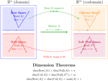
Geometric Visualization: The Four Fundamental Subspaces.

For a deeper understanding, we introduce a fourth fundamental subspace: the left null space \(\operatorname{Null}(A^T)\text{,}\) which is the null space of \(A^T\text{.}\) Together, these four subspaces form one of the most beautiful structures in linear algebra.

🔗

Figure 4.4.5. The Four Fundamental Subspaces of an \(m \times n\) matrix \(A\) (with rank \(r\))
🔗

The four fundamental subspaces of an \(m \times n\) matrix \(A\) with rank \(r\) are:

Row Space \(\operatorname{Row}(A)\text{:}\) Subspace of \(\mathbb{R}^n\) spanned by rows of \(A\text{.}\) Dimension = \(r\text{.}\)

🔗
Null Space \(\operatorname{Null}(A)\text{:}\) Subspace of \(\mathbb{R}^n\) of vectors that map to \(\mathbf{0}\text{.}\) Dimension = \(n-r\text{.}\)

🔗
Column Space \(\operatorname{Col}(A)\text{:}\) Subspace of \(\mathbb{R}^m\) spanned by columns of \(A\text{.}\) This is the range of \(A\text{.}\) Dimension = \(r\text{.}\)

🔗
Left Null Space \(\operatorname{Null}(A^T)\text{:}\) Subspace of \(\mathbb{R}^m\) of vectors \(\mathbf{y}\) such that \(A^T\mathbf{y} = \mathbf{0}\) (equivalently, \(\mathbf{y}^TA = \mathbf{0}^T\text{,}\) hence "left" null space). Dimension = \(m-r\text{.}\)

🔗

🔗

Insight 4.4.6. The Beautiful Structure of the Four Subspaces.

Orthogonal complements:
- In \(\mathbb{R}^n\text{:}\) \(\operatorname{Row}(A) \perp \operatorname{Null}(A)\text{.}\) Every vector in \(\operatorname{Row}(A)\) is orthogonal to every vector in \(\operatorname{Null}(A)\text{,}\) and together they fill all of \(\mathbb{R}^n\text{.}\)
  
  🔗
- In \(\mathbb{R}^m\text{:}\) \(\operatorname{Col}(A) \perp \operatorname{Null}(A^T)\text{.}\) Together they fill all of \(\mathbb{R}^m\text{.}\)
  
  🔗
🔗
Dimension relationships:
- \(\dim(\operatorname{Row}(A)) + \dim(\operatorname{Null}(A)) = n\) (Rank-Nullity Theorem)
  
  🔗
- \(\displaystyle \dim(\operatorname{Col}(A)) + \dim(\operatorname{Null}(A^T)) = m\)
  
  🔗
- \(\displaystyle \dim(\operatorname{Row}(A)) = \dim(\operatorname{Col}(A)) = \operatorname{rank}(A)\)
  
  🔗
🔗
How \(A\) acts:
- \(A\) maps \(\operatorname{Row}(A)\) onto \(\operatorname{Col}(A)\) (one-to-one and onto)
  
  🔗
- \(A\) maps \(\operatorname{Null}(A)\) to the zero vector \(\mathbf{0}\)
  
  🔗
- Every vector \(\mathbf{x} \in \mathbb{R}^n\) can be uniquely decomposed as \(\mathbf{x} = \mathbf{x}_r + \mathbf{x}_n\) where \(\mathbf{x}_r \in \operatorname{Row}(A)\) and \(\mathbf{x}_n \in \operatorname{Null}(A)\)
  
  🔗
🔗
Geometric interpretation: The four subspaces divide \(\mathbb{R}^n\) and \(\mathbb{R}^m\) into orthogonal components that fully describe how the matrix transformation \(A\) acts. The rank \(r\) measures the "effective dimension" of the transformation—how much of the domain maps to a non-zero output.

🔗

🔗

Example 4.4.7. A Simple Example.

Consider the matrix

🔗

\begin{equation*} A = \begin{bmatrix} 1 & 2 & 3 \\ 2 & 4 & 6 \end{bmatrix} \end{equation*}

🔗

Describe the three fundamental subspaces.

🔗

Solution.

Row Space:

🔗

\begin{equation*} \operatorname{Row}(A) = \operatorname{span}\left\{\begin{bmatrix}1\\2\\3\end{bmatrix}, \begin{bmatrix}2\\4\\6\end{bmatrix}\right\} \end{equation*}

🔗

Note that the second row is \(2\) times the first row, so these vectors are linearly dependent:

🔗

\begin{equation*} \operatorname{Row}(A) = \operatorname{span}\left\{\begin{bmatrix}1\\2\\3\end{bmatrix}\right\} \end{equation*}

🔗

This is a line through the origin in \(\mathbb{R}^3\text{.}\)

🔗

Column Space:

🔗

\begin{equation*} \operatorname{Col}(A) = \operatorname{span}\left\{\begin{bmatrix}1\\2\end{bmatrix}, \begin{bmatrix}2\\4\end{bmatrix}, \begin{bmatrix}3\\6\end{bmatrix}\right\} \end{equation*}

🔗

All three columns are multiples of \(\begin{bmatrix}1\\2\end{bmatrix}\text{,}\) so:

🔗

\begin{equation*} \operatorname{Col}(A) = \operatorname{span}\left\{\begin{bmatrix}1\\2\end{bmatrix}\right\} \end{equation*}

🔗

This is a line through the origin in \(\mathbb{R}^2\text{.}\)

🔗

Null Space: We solve \(A\mathbf{x} = \mathbf{0}\text{:}\)

🔗

\begin{equation*} \begin{bmatrix}1 & 2 & 3\\2 & 4 & 6\end{bmatrix}\begin{bmatrix}x_1\\x_2\\x_3\end{bmatrix} = \begin{bmatrix}0\\0\end{bmatrix} \end{equation*}

🔗

This gives us \(x_1 + 2x_2 + 3x_3 = 0\text{,}\) or \(x_1 = -2x_2 - 3x_3\text{.}\) Setting \(x_2 = s\) and \(x_3 = t\text{,}\) we get:

🔗

\begin{equation*} \mathbf{x} = \begin{bmatrix}-2s-3t\\s\\t\end{bmatrix} = s\begin{bmatrix}-2\\1\\0\end{bmatrix} + t\begin{bmatrix}-3\\0\\1\end{bmatrix} \end{equation*}

🔗

Therefore:

🔗

\begin{equation*} \operatorname{Null}(A) = \operatorname{span}\left\{\begin{bmatrix}-2\\1\\0\end{bmatrix}, \begin{bmatrix}-3\\0\\1\end{bmatrix}\right\} \end{equation*}

🔗

This is a plane through the origin in \(\mathbb{R}^3\text{.}\)

🔗

Subsection 4.4.2 Looking Ahead: Bases and Rank

Understanding these three subspaces is just the beginning. The next crucial questions are:

🔗

How do we find a basis for each subspace? Given a matrix \(A\text{,}\) we need systematic methods to find bases for \(\operatorname{Row}(A)\text{,}\) \(\operatorname{Col}(A)\text{,}\) and \(\operatorname{Null}(A)\text{.}\) Note that the three spaces can be described as a span of vectors, even through it is not obvious about the null space.
🔗

We define a basis of the subspaces as a set of vectors that both spans the subspace and is linearly independent. Finding such bases is essential for understanding the structure of these spaces. The dimension of a subspace is the number of vectors in a basis for the subspace.
🔗

🔗
What are the dimensions of these subspaces? The dimensions provide crucial information about the matrix. In particular:
- \(\dim(\operatorname{Row}(A))\) = ?
  
  🔗
- \(\dim(\operatorname{Col}(A))\) = ?
  
  🔗
- \(\dim(\operatorname{Null}(A))\) = ?
  
  🔗
🔗
🔗
How are these dimensions related? It turns out there are beautiful relationships between these dimensions. Most importantly:
- \(\dim(\operatorname{Row}(A)) = \dim(\operatorname{Col}(A))\) (this common value is called the rank of \(A\))
  
  🔗
- \(\text{rank}(A) + \dim(\operatorname{Null}(A)) = n\) (the Rank-Nullity Theorem)
  
  🔗
🔗
🔗

🔗

In the next subsection, we will develop systematic methods to find bases for these three fundamental subspaces and explore the concept of matrix rank. These tools are essential for both theoretical understanding and practical computation in linear algebra.

🔗

Subsection 4.4.3 Preliminary Exploration

Before we develop the systematic methods, let’s explore these concepts with some theoretical and computational activities.

🔗

Activity 4.4.1. Rank Invariance Under Right Multiplication.

Suppose \(A\) is an \(m \times n\) matrix, \(P\) is an \(n \times n\) invertible matrix, and \(B = AP\text{.}\) Prove that \(\operatorname{rank}(B) = \operatorname{rank}(A)\text{.}\)

🔗

Hint.

Consider the column spaces of \(A\) and \(B\text{.}\) Recall that the columns of \(B = AP\) are linear combinations of the columns of \(A\text{.}\) Use the fact that \(P\) is invertible to show that any linear combination of columns of \(A\) can be expressed as a linear combination of columns of \(B\text{,}\) and vice versa.

🔗

Solution.

We prove that \(\operatorname{Col}(A) = \operatorname{Col}(B)\text{,}\) which immediately implies \(\operatorname{rank}(A) = \operatorname{rank}(B)\text{.}\)

🔗

First, show \(\operatorname{Col}(B) \subseteq \operatorname{Col}(A)\text{:}\)

🔗

Let \(P = [\mathbf{p}_1 \; \mathbf{p}_2 \; \cdots \; \mathbf{p}_n]\) where \(\mathbf{p}_j \in \mathbb{R}^n\text{.}\) Then the \(j\)-th column of \(B = AP\) is:

🔗

\begin{equation*} \mathbf{b}_j = A\mathbf{p}_j. \end{equation*}

🔗

This shows that each column of \(B\) is in \(\operatorname{Col}(A)\text{.}\) Therefore, \(\operatorname{Col}(B) \subseteq \operatorname{Col}(A)\text{.}\)

🔗

Second, show \(\operatorname{Col}(A) \subseteq \operatorname{Col}(B)\text{:}\)

🔗

Since \(B = AP\) and \(P\) is invertible, we have \(A = BP^{-1}\text{.}\) By the same argument as above, each column of \(A\) is a linear combination of the columns of \(B\text{.}\) Therefore, \(\operatorname{Col}(A) \subseteq \operatorname{Col}(B)\text{.}\)

🔗

Since \(\operatorname{Col}(A) \subseteq \operatorname{Col}(B)\) and \(\operatorname{Col}(B) \subseteq \operatorname{Col}(A)\text{,}\) we conclude that \(\operatorname{Col}(A) = \operatorname{Col}(B)\text{.}\) Hence:

🔗

\begin{equation*} \operatorname{rank}(B) = \dim(\operatorname{Col}(B)) = \dim(\operatorname{Col}(A)) = \operatorname{rank}(A). \end{equation*}

🔗

Checkpoint 4.4.8. Rank Invariance Under Left Multiplication.

Suppose \(A\) is an \(m \times n\) matrix, \(Q\) is an \(m \times m\) invertible matrix, and \(B = QA\text{.}\) Prove that \(\operatorname{rank}(B) = \operatorname{rank}(A)\text{.}\)

🔗

Hint.

Consider the row spaces of \(A\) and \(B\text{.}\) The rows of \(B\) are linear combinations of the rows of \(A\text{.}\) Use the fact that \(Q\) is invertible to establish that \(\operatorname{Row}(A) = \operatorname{Row}(B)\text{.}\) Alternatively, you could use the fact that \(\operatorname{rank}(A) = \operatorname{rank}(A^T)\) and apply the result from Activity 4.4.1.

🔗

Solution.

Method 1: Using Row Spaces

🔗

We prove that \(\operatorname{Row}(A) = \operatorname{Row}(B)\text{.}\)

🔗

Since \(B = QA\text{,}\) each row of \(B\) is a linear combination of the rows of \(A\text{.}\) Therefore, \(\operatorname{Row}(B) \subseteq \operatorname{Row}(A)\text{.}\)

🔗

Conversely, since \(Q\) is invertible, we have \(A = Q^{-1}B\text{.}\) By the same reasoning, each row of \(A\) is a linear combination of the rows of \(B\text{.}\) Therefore, \(\operatorname{Row}(A) \subseteq \operatorname{Row}(B)\text{.}\)

🔗

Thus \(\operatorname{Row}(A) = \operatorname{Row}(B)\text{,}\) which implies:

🔗

\begin{equation*} \operatorname{rank}(B) = \dim(\operatorname{Row}(B)) = \dim(\operatorname{Row}(A)) = \operatorname{rank}(A). \end{equation*}

🔗

Method 2: Using Transpose

🔗

We have \(B = QA\text{,}\) so \(B^T = A^T Q^T\text{.}\) Since \(Q^T\) is invertible (being the transpose of an invertible matrix), Activity 4.4.1 tells us that:

🔗

\begin{equation*} \operatorname{rank}(B^T) = \operatorname{rank}(A^T). \end{equation*}

🔗

Since \(\operatorname{rank}(M) = \operatorname{rank}(M^T)\) for any matrix \(M\text{,}\) we conclude:

🔗

\begin{equation*} \operatorname{rank}(B) = \operatorname{rank}(B^T) = \operatorname{rank}(A^T) = \operatorname{rank}(A). \end{equation*}

🔗

These results show that multiplying by an invertible matrix (on either side) preserves the rank. This is a fundamental property that we will use repeatedly when studying matrix equivalence and similarity.

🔗

Activity 4.4.2. Exploring the Dimensions.

In this activity, we explore the dimensions of the row, column, and null spaces of a matrix. Use the Sage code below to investigate.

🔗

Discussion: Answer the questions below based on your computations.

The dimension of the row space is \(\underline{\qquad\qquad}\text{.}\)
🔗

Hint: This equals the number of nonzero rows in the reduced row echelon form (RREF) of \(A\text{,}\) which also equals the number of pivot columns in \(A\text{.}\)
🔗

🔗
The dimension of the column space is \(\underline{\qquad\qquad}\text{.}\)
🔗

Hint: This equals the number of pivot columns in \(A\text{,}\) which also equals the number of nonzero rows in the RREF of \(A\text{.}\)
🔗

🔗
The dimension of the null space is \(\underline{\qquad\qquad}\text{.}\)
🔗

Hint: This equals the number of free variables in the system \(A\mathbf{x}=\mathbf{0}\text{,}\) which equals (number of columns) minus (number of pivot columns).
🔗

🔗
Key Observation: What do you notice about the relationship between:
- \(\dim(\operatorname{Row}(A))\) and \(\dim(\operatorname{Col}(A))\text{?}\)
  
  🔗
- \(\dim(\operatorname{Row}(A)) + \dim(\operatorname{Null}(A))\) and the number of columns of \(A\text{?}\)
  
  🔗
🔗
🔗

🔗

Subsection 4.4.4 Finding Bases for Row, Column, and Null Spaces

Now that we understand what row spaces, column spaces, and null spaces are, a natural question arises: How do we find a basis for each of these spaces? This is a fundamental computational problem in linear algebra, and fortunately, we have systematic methods for solving it.

🔗

Methods for Finding Bases.

Let \(A\) be an \(m \times n\) matrix. Let \(R\) denote the reduced row echelon form (RREF) of \(A\text{.}\)

🔗

1. Basis for the Row Space \(\operatorname{Row}(A)\text{:}\)

🔗

The nonzero rows of the RREF \(R\) form a basis for \(\operatorname{Row}(A)\text{.}\)

🔗

Why? Row operations do not change the row space, and the nonzero rows of \(R\) are linearly independent.

🔗

2. Basis for the Column Space \(\operatorname{Col}(A)\text{:}\)

🔗

The columns of \(A\) that correspond to the pivot columns in \(R\) form a basis for \(\operatorname{Col}(A)\text{.}\)

🔗

Important: We take the columns from the original matrix \(A\text{,}\) not from \(R\text{!}\)

🔗

Why? Row operations preserve linear dependence relationships among columns, but they change the column space itself. The pivot columns of \(R\) identify which columns of \(A\) are linearly independent.

🔗

3. Basis for the Null Space \(\operatorname{Null}(A)\text{:}\)

🔗

Solve the homogeneous system \(A\mathbf{x} = \mathbf{0}\) (or equivalently \(R\mathbf{x} = \mathbf{0}\)) by expressing the basic variables in terms of the free variables. Each free variable gives rise to one basic solution vector, and these basic solution vectors form a basis for \(\operatorname{Null}(A)\text{.}\)

🔗

Example 4.4.9. Finding Bases for Row, Column, and Null Spaces.

Let

🔗

\begin{equation*} A = \begin{bmatrix} 1 & 3 & 1 & 3 \\ 0 & 1 & 1 & 0 \\ 1 & 5 & 3 & 3 \\ -3 & 0 & 6 & -1 \\ 3 & 4 & -2 & 1 \end{bmatrix} \end{equation*}

🔗

Find a basis for each of the following:

\(\displaystyle \operatorname{Row}(A)\)

🔗
\(\displaystyle \operatorname{Col}(A)\)

🔗
\(\displaystyle \operatorname{Null}(A)\)

🔗

🔗

Solution.

Step 1: Find the RREF of \(A\)

🔗

From the computation, we get the RREF:

🔗

\begin{equation*} R = \begin{bmatrix} 1 & 0 & -2 & 0 \\ 0 & 1 & 1 & 0 \\ 0 & 0 & 0 & 1 \\ 0 & 0 & 0 & 0 \\ 0 & 0 & 0 & 0 \end{bmatrix} \end{equation*}

🔗

The pivot columns are columns 1, 2, and 4.

🔗

Part 1: Basis for \(\operatorname{Row}(A)\)

🔗

The nonzero rows of \(R\) form a basis for \(\operatorname{Row}(A)\text{:}\)

🔗

\begin{equation*} \text{Basis for } \operatorname{Row}(A) = \left\{\begin{bmatrix}1\\0\\-2\\0\end{bmatrix}, \begin{bmatrix}0\\1\\1\\0\end{bmatrix}, \begin{bmatrix}0\\0\\0\\1\end{bmatrix}\right\} \end{equation*}

🔗

Therefore, \(\dim(\operatorname{Row}(A)) = 3\text{.}\)

🔗

Part 2: Basis for \(\operatorname{Col}(A)\)

🔗

The pivot columns are columns 1, 2, and 4. We take the corresponding columns from the original matrix \(A\text{:}\)

🔗

\begin{equation*} \text{Basis for } \operatorname{Col}(A) = \left\{\begin{bmatrix}1\\0\\1\\-3\\3\end{bmatrix}, \begin{bmatrix}3\\1\\5\\0\\4\end{bmatrix}, \begin{bmatrix}3\\0\\3\\-1\\1\end{bmatrix}\right\} \end{equation*}

🔗

Therefore, \(\dim(\operatorname{Col}(A)) = 3\text{.}\)

🔗

Important Observation: Notice that \(\dim(\operatorname{Row}(A)) = \dim(\operatorname{Col}(A)) = 3\text{.}\) This is not a coincidence! This common dimension is called the rank of the matrix \(A\text{.}\)

🔗

Part 3: Basis for \(\operatorname{Null}(A)\)

🔗

We need to solve \(A\mathbf{x} = \mathbf{0}\text{,}\) or equivalently, \(R\mathbf{x} = \mathbf{0}\text{.}\)

🔗

From the RREF, we have:

\begin{align*} x_1 - 2x_3 &= 0\\ x_2 + x_3 &= 0\\ x_4 &= 0 \end{align*}

🔗

The free variable is \(x_3\text{.}\) Expressing the basic variables in terms of the free variable:

\begin{align*} x_1 &= 2x_3\\ x_2 &= -x_3\\ x_3 &= x_3 \text{ (free)}\\ x_4 &= 0 \end{align*}

🔗

Setting \(x_3 = t\text{,}\) we get:

🔗

\begin{equation*} \mathbf{x} = \begin{bmatrix}2t\\-t\\t\\0\end{bmatrix} = t\begin{bmatrix}2\\-1\\1\\0\end{bmatrix} \end{equation*}

🔗

Therefore, a basis for \(\operatorname{Null}(A)\) is:

🔗

\begin{equation*} \text{Basis for } \operatorname{Null}(A) = \left\{\begin{bmatrix}2\\-1\\1\\0\end{bmatrix}\right\} \end{equation*}

🔗

Therefore, \(\dim(\operatorname{Null}(A)) = 1\text{.}\)

🔗

Summary:

🔗

\(\operatorname{Row}(A)\) has dimension 3, with basis formed by the nonzero rows of RREF

🔗
\(\operatorname{Col}(A)\) has dimension 3, with basis formed by columns 1, 2, and 4 of \(A\)

🔗
\(\operatorname{Null}(A)\) has dimension 1, with basis formed by the basic solution vector

🔗
Notice: \(\text{rank}(A) + \text{nullity}(A) = 3 + 1 = 4 = n\) (the Rank-Nullity Theorem!)

🔗

🔗

Activity 4.4.3. Practice: Finding Bases.

Let

🔗

\begin{equation*} B = \begin{bmatrix} -2 & -5 & 8 & 0 & -17 \\ 1 & 3 & -5 & 1 & 5 \\ 3 & 11 & -19 & 7 & 1 \\ 1 & 7 & -13 & 5 & -3 \end{bmatrix} \end{equation*}

🔗

Find a basis for each of the following:

\(\displaystyle \operatorname{Row}(B)\)

🔗
\(\displaystyle \operatorname{Col}(B)\)

🔗
\(\displaystyle \operatorname{Null}(B)\)

🔗

Also verify the Rank-Nullity Theorem for this matrix.

🔗

Hint.

Follow the same steps as in the example:

Compute the RREF of \(B\)

🔗
Identify the pivot columns

🔗
For row space: use nonzero rows of RREF

🔗
For column space: use corresponding columns from \(B\) (not RREF!)

🔗
For null space: solve \(B\mathbf{x} = \mathbf{0}\) and express in terms of free variables

🔗

🔗

Solution.

🔗

Insight 4.4.10. Common Misconception: Can We Use the First Few Rows?

Question: In our example with matrix \(A\text{,}\) we found that \(\dim(\operatorname{Row}(A)) = 3\text{.}\) Since \(A\) has 5 rows, can we simply take the first three rows of \(A\) as a basis for \(\operatorname{Row}(A)\text{?}\)

🔗

Answer: NO! This is a common mistake. Let’s see why.

🔗

The first three rows of \(A\) are:

🔗

\begin{equation*} \mathbf{r}_1 = \begin{bmatrix}1 & 3 & 1 & 3\end{bmatrix}, \quad \mathbf{r}_2 = \begin{bmatrix}0 & 1 & 1 & 0\end{bmatrix}, \quad \mathbf{r}_3 = \begin{bmatrix}1 & 5 & 3 & 3\end{bmatrix} \end{equation*}

🔗

Problem 1: These might not be linearly independent!

🔗

The Key Issue:

🔗

Even if the first \(k\) rows happen to be linearly independent (where \(k = \text{rank}(A)\)), they might not span the entire row space! The row space is determined by all the rows of the matrix, not just the first few.

🔗

For example, consider a matrix where the first three rows are linearly independent, but the fourth row contains crucial information that cannot be expressed as a linear combination of the first three. The first three rows would not span the row space, even though they are linearly independent.

🔗

The Safe Method:

🔗

Always compute the RREF

🔗
Use the nonzero rows of RREF as a basis for the row space

🔗
This guarantees both linear independence AND that they span the correct space

🔗

🔗

Why RREF Works:

🔗

Row operations preserve the row space: \(\operatorname{Row}(A) = \operatorname{Row}(R)\)

🔗
The nonzero rows of RREF are in a special form that makes their linear independence obvious

🔗
Together, these facts guarantee that the nonzero rows of RREF form a basis

🔗

🔗

Prev Top Next