
Section 6.4 Properties of Linear Transformations

In this section, we study important properties of linear transformations that determine their behavior: whether they are one-to-one, onto, or invertible. These concepts help us understand when and how linear transformations can be "reversed" and how they can be combined.

Subsection 6.4.1 One-to-One and Onto Transformations

Definition 6.4.1. One-to-One and Onto.

Let \(T: V \rightarrow W\) be a linear transformation.
  1. \(T\) is called one-to-one (or injective) if different vectors in \(V\) are mapped to different vectors in \(W\text{.}\) That is,
    \begin{equation*} T(\mathbf{u}) = T(\mathbf{v}) \implies \mathbf{u} = \mathbf{v} \end{equation*}
    for all \(\mathbf{u}, \mathbf{v} \in V\text{.}\)
    Equivalently, \(T\) is one-to-one if and only if \(T(\mathbf{v}) = \mathbf{0}\) implies \(\mathbf{v} = \mathbf{0}\text{.}\)
  2. \(T\) is called onto (or surjective) if every vector in \(W\) is the image of at least one vector in \(V\text{.}\) That is,
    \begin{equation*} \text{for every } \mathbf{w} \in W, \text{ there exists } \mathbf{v} \in V \text{ such that } T(\mathbf{v}) = \mathbf{w}. \end{equation*}
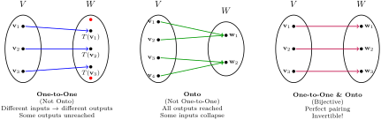
    Equivalently, \(T\) is onto if and only if \(\operatorname{range}(T) = W\text{.}\)

Geometric Interpretation.

  • One-to-One: Think of \(T\) as a transformation that never collapses distinct points together. If two points are different before the transformation, they remain different after. Geometrically, \(T\) preserves distinctness — no "squashing" occurs.
    Example: A rotation or reflection in \(\mathbb{R}^2\) is one-to-one because distinct points don’t overlap.
  • Onto: Think of \(T\) as a transformation that fills up the entire target space \(W\text{.}\) Every point in \(W\) is "hit" by the transformation. Geometrically, \(T\) covers all of \(W\) — no gaps remain.
    Example: A projection from \(\mathbb{R}^3\) to \(\mathbb{R}^2\) can be onto because it covers the entire plane.
described in detail following the image
Illustrates the difference between one-to-one and onto transformations using mapping diagrams.
Figure 6.4.2. Visual Comparison: One-to-One vs Onto

Example 6.4.3. A Transformation Neither One-to-One Nor Onto.

Consider the linear transformation \(T:\mathbb{R}^{4}\rightarrow \mathbb{R}^{4}\) from Example 6.1.4. We showed that:
  • \(\displaystyle \operatorname{ker}(T) = \operatorname{span}\left\{\begin{pmatrix}-2\\2\\-1\\1\end{pmatrix}\right\} \neq \{\mathbf{0}\}\)
  • \(\operatorname{range}(T) = \operatorname{span}\left\{\begin{pmatrix}1\\0\\-1\\0\end{pmatrix}, \begin{pmatrix}1\\1\\0\\2\end{pmatrix}, \begin{pmatrix}0\\3\\1\\2\end{pmatrix}\right\}\text{,}\) which is a proper subspace of \(\mathbb{R}^4\)
Therefore:
  • \(T\) is not one-to-one because \(\operatorname{ker}(T) \neq \{\mathbf{0}\}\text{.}\) For instance, \(T\begin{pmatrix}-2\\2\\-1\\1\end{pmatrix} = \mathbf{0} = T(\mathbf{0})\text{,}\) but \(\begin{pmatrix}-2\\2\\-1\\1\end{pmatrix} \neq \mathbf{0}\text{.}\)
  • \(T\) is not onto because \(\operatorname{range}(T) \neq \mathbb{R}^4\text{.}\) In fact, \(\dim(\operatorname{range}(T)) = 3 < 4 = \dim(\mathbb{R}^4)\text{,}\) so there exist vectors in \(\mathbb{R}^4\) that are not in the range of \(T\text{.}\)

Proof.

(\(\Rightarrow\)) Assume \(T\) is one-to-one. We know \(\mathbf{0} \in \operatorname{ker}(T)\) because \(T(\mathbf{0}) = \mathbf{0}\text{.}\) Suppose \(\mathbf{v} \in \operatorname{ker}(T)\text{.}\) Then \(T(\mathbf{v}) = \mathbf{0} = T(\mathbf{0})\text{.}\) Since \(T\) is one-to-one, we must have \(\mathbf{v} = \mathbf{0}\text{.}\) Therefore, \(\operatorname{ker}(T) = \{\mathbf{0}\}\text{.}\)
(\(\Leftarrow\)) Assume \(\operatorname{ker}(T) = \{\mathbf{0}\}\text{.}\) Suppose \(T(\mathbf{u}) = T(\mathbf{v})\text{.}\) Then
\begin{equation*} T(\mathbf{u}) - T(\mathbf{v}) = \mathbf{0} \implies T(\mathbf{u} - \mathbf{v}) = \mathbf{0} \implies \mathbf{u} - \mathbf{v} \in \operatorname{ker}(T). \end{equation*}
Since \(\operatorname{ker}(T) = \{\mathbf{0}\}\text{,}\) we have \(\mathbf{u} - \mathbf{v} = \mathbf{0}\text{,}\) so \(\mathbf{u} = \mathbf{v}\text{.}\) Therefore, \(T\) is one-to-one.

Example 6.4.5. Checking One-to-One.

Determine whether the linear transformation \(T: \mathbb{R}^3 \rightarrow \mathbb{R}^3\) defined by
\begin{equation*} T\left(\begin{bmatrix} x_1 \\ x_2 \\ x_3 \end{bmatrix}\right) = \begin{bmatrix} x_1 + x_2 \\ x_2 + x_3 \\ x_1 + x_3 \end{bmatrix} \end{equation*}
is one-to-one.
Solution.
By Theorem 6.4.4, \(T\) is one-to-one if and only if \(\operatorname{ker}(T) = \{\mathbf{0}\}\text{.}\) We need to solve \(T(\mathbf{x}) = \mathbf{0}\text{:}\)
\begin{equation*} \begin{bmatrix} x_1 + x_2 \\ x_2 + x_3 \\ x_1 + x_3 \end{bmatrix} = \begin{bmatrix} 0 \\ 0 \\ 0 \end{bmatrix} \end{equation*}
This gives the system:
\begin{align*} x_1 + x_2 \amp= 0\\ x_2 + x_3 \amp= 0\\ x_1 + x_3 \amp= 0 \end{align*}
The augmented matrix for this system is:
\begin{equation*} \left[\begin{array}{ccc|c} 1 \amp 1 \amp 0 \amp 0 \\ 0 \amp 1 \amp 1 \amp 0 \\ 1 \amp 0 \amp 1 \amp 0 \end{array}\right]\xrightarrow{\operatorname{RREF}}\left[\begin{array}{ccc|c} 1 \amp 0 \amp 0 \amp 0 \\ 0 \amp 1 \amp 0 \amp 0 \\ 0 \amp 0 \amp 1 \amp 0 \end{array}\right] \end{equation*}
Therefore, the unique solution is \(x_1 = x_2 = x_3 = 0\text{.}\)
Since \(\operatorname{ker}(T) = \{\mathbf{0}\}\text{,}\) the transformation \(T\) is one-to-one.

Proof.

By definition, \(T\) is onto if and only if \(\operatorname{range}(T) = W\text{.}\) Since \(W\) is finite-dimensional, this occurs if and only if \(\dim(\operatorname{range}(T)) = \dim(W)\text{.}\)

Example 6.4.7. The Transformation from Example 6.4.5 is Also Onto.

Show that the linear transformation \(T: \mathbb{R}^3 \rightarrow \mathbb{R}^3\) from Example 6.4.5 is also onto.
Solution.
By Theorem 6.4.6, \(T\) is onto if and only if \(\dim(\operatorname{range}(T)) = \dim(\mathbb{R}^3) = 3\text{.}\) The standard matrix for \(T\) is
\begin{equation*} A = \begin{bmatrix} 1 \amp 1 \amp 0 \\ 0 \amp 1 \amp 1 \\ 1 \amp 0 \amp 1 \end{bmatrix}. \end{equation*}
In Example 6.4.5, we showed that \(\dim(\operatorname{ker}(T)) = 0\text{.}\) By the Rank-Nullity Theorem,
\begin{equation*} \dim(\operatorname{range}(T)) = \dim(\mathbb{R}^3) - \dim(\operatorname{ker}(T)) = 3 - 0 = 3. \end{equation*}
Since \(\dim(\operatorname{range}(T)) = 3 = \dim(\mathbb{R}^3)\text{,}\) the transformation \(T\) is onto.

Example 6.4.8. Checking Onto.

Determine whether the linear transformation \(T: \mathbb{R}^3 \rightarrow \mathbb{R}^2\) defined by
\begin{equation*} T\left(\begin{bmatrix} x_1 \\ x_2 \\ x_3 \end{bmatrix}\right) = \begin{bmatrix} x_1 + x_2 \\ x_2 + x_3 \end{bmatrix} \end{equation*}
is onto.
Solution.
By Theorem 6.4.6, \(T\) is onto if and only if \(\dim(\operatorname{range}(T)) = \dim(\mathbb{R}^2) = 2\text{.}\) The standard matrix for \(T\) is
\begin{equation*} A = \begin{bmatrix} 1 \amp 1 \amp 0 \\ 0 \amp 1 \amp 1 \end{bmatrix}. \end{equation*}
Since \(\operatorname{range}(T) = \operatorname{Col}(A)\text{,}\) we need to find the dimension of the column space of \(A\text{.}\)
Row reducing \(A\) to row echelon form:
\begin{equation*} \begin{bmatrix} 1 \amp 1 \amp 0 \\ 0 \amp 1 \amp 1 \end{bmatrix} \end{equation*}
The matrix is already in row echelon form with two pivot positions (in columns 1 and 2). Therefore, \(\dim(\operatorname{Col}(A)) = 2\text{.}\)
Since \(\dim(\operatorname{range}(T)) = 2 = \dim(\mathbb{R}^2)\text{,}\) the transformation \(T\) is onto.

Subsection 6.4.2 Invertible Linear Transformations

Definition 6.4.9. Invertible Transformation.

A linear transformation \(T: V \rightarrow W\) is called invertible if there exists a linear transformation \(S: W \rightarrow V\) such that
\begin{equation*} S \circ T = I_V \quad \text{and} \quad T \circ S = I_W, \end{equation*}
where \(I_V\) and \(I_W\) are the identity transformations on \(V\) and \(W\text{,}\) respectively.
The transformation \(S\) is called the inverse of \(T\text{,}\) denoted \(T^{-1}\text{.}\)

Proof.

(\(\Rightarrow\)) Assume \(T\) is invertible with inverse \(T^{-1}\text{.}\)
One-to-one: If \(T(\mathbf{u}) = T(\mathbf{v})\text{,}\) then applying \(T^{-1}\) to both sides gives
\begin{equation*} T^{-1}(T(\mathbf{u})) = T^{-1}(T(\mathbf{v})) \implies \mathbf{u} = \mathbf{v}. \end{equation*}
So \(T\) is one-to-one.
Onto: For any \(\mathbf{w} \in W\text{,}\) let \(\mathbf{v} = T^{-1}(\mathbf{w})\text{.}\) Then
\begin{equation*} T(\mathbf{v}) = T(T^{-1}(\mathbf{w})) = \mathbf{w}. \end{equation*}
So \(T\) is onto.
(\(\Leftarrow\)) Assume \(T\) is both one-to-one and onto. For each \(\mathbf{w} \in W\text{,}\) since \(T\) is onto, there exists at least one \(\mathbf{v} \in V\) such that \(T(\mathbf{v}) = \mathbf{w}\text{.}\) Since \(T\) is one-to-one, this \(\mathbf{v}\) is unique. Define \(T^{-1}(\mathbf{w}) = \mathbf{v}\text{.}\) One can verify that \(T^{-1}\) is linear and satisfies the inverse properties.

Proof.

By Theorem 6.4.10, \(T\) is invertible if and only if \(T\) is both one-to-one and onto.
(\(\Rightarrow\)) Assume \(T\) is invertible. Then \(T\) is one-to-one, so \(\operatorname{ker}(T) = \{\mathbf{0}\}\text{.}\) This means the only solution to \([T]_\alpha^\beta [\mathbf{x}]_\alpha = \mathbf{0}\) is \([\mathbf{x}]_\alpha = \mathbf{0}\text{.}\) Therefore, the columns of \([T]_\alpha^\beta\) are linearly independent. Since \([T]_\alpha^\beta\) is an \(n \times n\) matrix with \(n\) linearly independent columns, it is invertible.
(\(\Leftarrow\)) Assume \([T]_\alpha^\beta\) is invertible. Then the columns of \([T]_\alpha^\beta\) are linearly independent, which implies \(\operatorname{ker}(T) = \{\mathbf{0}\}\text{,}\) so \(T\) is one-to-one. By the Rank-Nullity Theorem,
\begin{equation*} \dim(\operatorname{range}(T)) = \dim(V) - \dim(\operatorname{ker}(T)) = n - 0 = n = \dim(W). \end{equation*}
By Theorem 6.4.6, \(T\) is onto. Since \(T\) is both one-to-one and onto, \(T\) is invertible.

Example 6.4.12.

Let \(T: \mathbb{R}^3 \rightarrow \mathbb{R}^3\) be a linear transformation such that
\begin{equation*} T\left(\begin{bmatrix} x \\ y \\ z \end{bmatrix}\right) = \begin{bmatrix}x-2y+z \\ 2x+2y-8z \\ 5x+y-5z\end{bmatrix}. \end{equation*}
Question: Is \(T\) invertible? If so, find \(T^{-1}\text{.}\)
Hint.
Use Theorem 6.4.11 to check if the standard matrix \(A\) is invertible. To find \(T^{-1}\text{,}\) compute the reduced row echelon form of the augmented matrix \([A \mid I]\text{,}\) where \(I\) is the \(3 \times 3\) identity matrix. If \(A\) is invertible, the RREF will be \([I \mid A^{-1}]\text{.}\)
Solution.
The standard matrix for \(T\) is
\begin{equation*} A = \begin{bmatrix} 1 \amp -2 \amp 1 \\ 2 \amp 2 \amp -8 \\ 5 \amp 1 \amp -5 \end{bmatrix}. \end{equation*}
By Theorem 6.4.11, \(T\) is invertible if and only if \(A\) is invertible.
We use SageMath to compute the reduced row echelon form of \([A \mid I]\text{:}\)
From the output, we see that the RREF is
\begin{equation*} \left[\begin{array}{ccc|ccc} 1 \amp 0 \amp 0 \amp -1 \amp -\frac{9}{2} \amp \frac{7}{2} \\ 0 \amp 1 \amp 0 \amp 15 \amp -5 \amp 5 \\ 0 \amp 0 \amp 1 \amp 4 \amp -\frac{11}{2} \amp \frac{3}{2} \end{array}\right]. \end{equation*}
Since the left side is the identity matrix, \(A\) is invertible. Therefore, \(T\) is invertible with inverse matrix
\begin{equation*} A^{-1} = \begin{bmatrix} -1 \amp -\frac{9}{2} \amp \frac{7}{2} \\ 15 \amp -5 \amp 5 \\ 4 \amp -\frac{11}{2} \amp \frac{3}{2} \end{bmatrix}. \end{equation*}
Thus, the inverse transformation is
\begin{equation*} T^{-1}\left(\begin{bmatrix} x \\ y \\ z \end{bmatrix}\right) = \begin{bmatrix} -x - \frac{9}{2}y + \frac{7}{2}z \\ 15x - 5y + 5z \\ 4x - \frac{11}{2}y + \frac{3}{2}z \end{bmatrix}. \end{equation*}

Checkpoint 6.4.13.

Let \(T: \mathbb{P}_2(x) \rightarrow \mathbb{P}_2(x)\) be a linear transformation such that
\begin{equation*} T\left(a+bx+cx^2\right) = (a-2b+c)+(2a+2b-8c)x+(5a+b-5c)x^2. \end{equation*}
Question: Is \(T\) invertible? If so, find \(T^{-1}(a+bx+cx^2)\text{.}\)

Example 6.4.14. Rotation is Invertible.

Consider the rotation transformation \(T: \mathbb{R}^2 \rightarrow \mathbb{R}^2\) that rotates vectors counterclockwise by \(\theta\) radians:
\begin{equation*} T\left(\begin{bmatrix} x \\ y \end{bmatrix}\right) = \begin{bmatrix} \cos\theta \amp -\sin\theta \\ \sin\theta \amp \cos\theta \end{bmatrix} \begin{bmatrix} x \\ y \end{bmatrix}. \end{equation*}
Show that \(T\) is invertible and find \(T^{-1}\text{.}\)
Solution.
The standard matrix is \(A = \begin{bmatrix} \cos\theta \amp -\sin\theta \\ \sin\theta \amp \cos\theta \end{bmatrix}\text{.}\) We compute
\begin{equation*} \det(A) = \cos^2\theta + \sin^2\theta = 1 \neq 0. \end{equation*}
Since \(\det(A) \neq 0\text{,}\) the matrix \(A\) is invertible, so \(T\) is invertible.
The inverse transformation rotates by \(-\theta\) (clockwise):
\begin{equation*} T^{-1}\left(\begin{bmatrix} x \\ y \end{bmatrix}\right) = \begin{bmatrix} \cos\theta \amp \sin\theta \\ -\sin\theta \amp \cos\theta \end{bmatrix} \begin{bmatrix} x \\ y \end{bmatrix}. \end{equation*}
Geometric interpretation: To undo a counterclockwise rotation by \(\theta\text{,}\) we rotate clockwise by \(\theta\text{.}\)

Example 6.4.15. Projection is Not Invertible.

Consider the projection \(T: \mathbb{R}^3 \rightarrow \mathbb{R}^3\) onto the \(xy\)-plane:
\begin{equation*} T\left(\begin{bmatrix} x \\ y \\ z \end{bmatrix}\right) = \begin{bmatrix} x \\ y \\ 0 \end{bmatrix}. \end{equation*}
Show that \(T\) is not invertible.
Solution.
To check if \(T\) is one-to-one, we find \(\operatorname{ker}(T)\text{:}\)
\begin{equation*} T\left(\begin{bmatrix} x \\ y \\ z \end{bmatrix}\right) = \begin{bmatrix} 0 \\ 0 \\ 0 \end{bmatrix} \implies \begin{bmatrix} x \\ y \\ 0 \end{bmatrix} = \begin{bmatrix} 0 \\ 0 \\ 0 \end{bmatrix} \implies x = y = 0. \end{equation*}
So \(\operatorname{ker}(T) = \left\{\begin{bmatrix} 0 \\ 0 \\ z \end{bmatrix} : z \in \mathbb{R}\right\}\text{,}\) which is the \(z\)-axis.
Since \(\operatorname{ker}(T) \neq \{\mathbf{0}\}\text{,}\) the transformation \(T\) is not one-to-one, hence not invertible.
Geometric interpretation: All points along a vertical line (parallel to the \(z\)-axis) project to the same point in the \(xy\)-plane. Information about the \(z\)-coordinate is lost, so the transformation cannot be reversed.

Insight 6.4.16. The Power of Matrix Representation.

Throughout this section, we have seen that the matrix representation of a linear transformation \(T: \mathbb{R}^n \rightarrow \mathbb{R}^m\) plays a crucial role in determining its properties. Once we identify the standard matrix \(A\) of \(T\text{,}\) many fundamental questions about the transformation reduce to questions about the matrix:
  • \(T\) is one-to-one if and only if the columns of \(A\) are linearly independent, which we can verify by checking that \(\operatorname{rank}(A) = n\text{.}\)
  • \(T\) is onto if and only if the columns of \(A\) span \(\mathbb{R}^m\text{,}\) which means \(\operatorname{rank}(A) = m\text{.}\)
  • \(T\) is invertible if and only if \(A\) is an invertible matrix, which for square matrices means \(\det(A) \neq 0\text{.}\)
  • The kernel of \(T\) is the null space of \(A\text{,}\) found by solving the homogeneous system \(A\mathbf{x} = \mathbf{0}\text{.}\)
  • The range of \(T\) is the column space of \(A\text{,}\) which is spanned by the pivot columns of \(A\text{.}\)
This connection between transformations and matrices is profound: it transforms abstract questions about functions between vector spaces into concrete computational problems involving systems of linear equations, row reduction, and matrix algebra. The matrix is not just a convenient representation—it is the key that unlocks our ability to analyze and compute with linear transformations systematically.

Subsection 6.4.3 Composition of Linear Transformations

Definition 6.4.17. Composition of Transformations.

Let \(T: U \rightarrow V\) and \(S: V \rightarrow W\) be linear transformations. The composition of \(S\) and \(T\text{,}\) denoted \(S \circ T\text{,}\) is the transformation from \(U\) to \(W\) defined by
\begin{equation*} (S \circ T)(\mathbf{u}) = S(T(\mathbf{u})) \end{equation*}
for all \(\mathbf{u} \in U\text{.}\)

Proof.

We need to verify the two properties of linearity. Let \(\mathbf{u}_1, \mathbf{u}_2 \in U\) and \(c \in \mathbb{R}\text{.}\)
Additivity:
\begin{align*} (S \circ T)(\mathbf{u}_1 + \mathbf{u}_2) \amp= S(T(\mathbf{u}_1 + \mathbf{u}_2))\\ \amp= S(T(\mathbf{u}_1) + T(\mathbf{u}_2)) \quad \text{(since } T \text{ is linear)}\\ \amp= S(T(\mathbf{u}_1)) + S(T(\mathbf{u}_2)) \quad \text{(since } S \text{ is linear)}\\ \amp= (S \circ T)(\mathbf{u}_1) + (S \circ T)(\mathbf{u}_2) \end{align*}
Homogeneity:
\begin{align*} (S \circ T)(c\mathbf{u}_1) \amp= S(T(c\mathbf{u}_1))\\ \amp= S(cT(\mathbf{u}_1)) \quad \text{(since } T \text{ is linear)}\\ \amp= cS(T(\mathbf{u}_1)) \quad \text{(since } S \text{ is linear)}\\ \amp= c(S \circ T)(\mathbf{u}_1) \end{align*}

Proof.

For any \(\mathbf{x} \in \mathbb{R}^n\text{,}\)
\begin{align*} (S \circ T)(\mathbf{x}) \amp= S(T(\mathbf{x}))\\ \amp= S(A\mathbf{x})\\ \amp= B(A\mathbf{x})\\ \amp= (BA)\mathbf{x} \end{align*}
Therefore, the standard matrix of \(S \circ T\) is \(BA\text{.}\)

Example 6.4.20. Composition: Rotation followed by Scaling.

Let \(T: \mathbb{R}^2 \rightarrow \mathbb{R}^2\) be the rotation by \(90°\) counterclockwise, and let \(S: \mathbb{R}^2 \rightarrow \mathbb{R}^2\) be the scaling that doubles all coordinates. Find the standard matrix of \(S \circ T\text{.}\)
Solution.
The standard matrices are:
\begin{equation*} A = \begin{bmatrix} 0 \amp -1 \\ 1 \amp 0 \end{bmatrix} \quad \text{(rotation by } 90°\text{)} \end{equation*}
\begin{equation*} B = \begin{bmatrix} 2 \amp 0 \\ 0 \amp 2 \end{bmatrix} \quad \text{(scaling by 2)} \end{equation*}
By Theorem 6.4.19, the standard matrix of \(S \circ T\) is
\begin{equation*} BA = \begin{bmatrix} 2 \amp 0 \\ 0 \amp 2 \end{bmatrix} \begin{bmatrix} 0 \amp -1 \\ 1 \amp 0 \end{bmatrix} = \begin{bmatrix} 0 \amp -2 \\ 2 \amp 0 \end{bmatrix}. \end{equation*}
Interpretation: First rotate by \(90°\text{,}\) then scale by 2. For example, \((S \circ T)\left(\begin{bmatrix} 1 \\ 0 \end{bmatrix}\right) = \begin{bmatrix} 0 \\ 2 \end{bmatrix}\text{.}\)

Warning 6.4.21. Order Matters!

Composition of transformations is not commutative: in general, \(S \circ T \neq T \circ S\text{.}\) The order in which transformations are applied matters!
For example, in Example 6.4.20, if we compute \(T \circ S\) (scale first, then rotate), we get
\begin{equation*} AB = \begin{bmatrix} 0 \amp -1 \\ 1 \amp 0 \end{bmatrix} \begin{bmatrix} 2 \amp 0 \\ 0 \amp 2 \end{bmatrix} = \begin{bmatrix} 0 \amp -2 \\ 2 \amp 0 \end{bmatrix}, \end{equation*}
1 which happens to be the same. But this is not always the case!

