
Section 7.1 Eigenvalues and Eigenvectors: Finding Special Directions

Recall from Chapter 6 that every \(n \times n\) matrix \(A\) defines a linear transformation \(T: \mathbb{R}^n \to \mathbb{R}^n\) by \(T(\mathbf{x}) = A\mathbf{x}\text{.}\) In general, this transformation can rotate, reflect, stretch, and shear vectors in complicated ways. But what if we could find special vectors that \(A\) only stretches (or compresses), without changing direction? In math language, to find a nonzero vector \(\mathbf{x}\) such that \(A\mathbf{x} = \lambda\mathbf{x}\) for some scalar \(\lambda\text{.}\) These special vectors would give us the clearest understanding of what \(A\) really does. This is the motivation for defining eigenvalues and eigenvectors, which give us a new lens to understand matrices.

Subsection 7.1.1 Definition of Eigenvalues and Eigenvectors

Definition 7.1.1. Eigenvalue and Eigenvector.

Let \(A\) be an \(n \times n\) matrix. A scalar \(\lambda\) (real number) is called an eigenvalue of \(A\) if there exists a nonzero vector \(\mathbf{x}\) such that
\begin{equation*} A\mathbf{x} = \lambda\mathbf{x} \end{equation*}
Any such nonzero vector \(\mathbf{x}\) is called an eigenvector of \(A\) corresponding to the eigenvalue \(\lambda\text{.}\)

Checkpoint 7.1.2. Verifying the Definition.

For each of the following, compute \(A\mathbf{v}\) directly. Verify that \(\mathbf{v}\) is an eigenvector of \(A\) according to Definition 7.1.1, and determine the corresponding eigenvalue \(\lambda\text{.}\)
(a)
\(A = \begin{bmatrix} 2 \amp -12 \\ 1 \amp -5 \end{bmatrix}\text{,}\) \(\mathbf{v} = \begin{bmatrix} 4 \\ 1 \end{bmatrix}\text{.}\)
Solution.
\begin{equation*} A\mathbf{v} = \begin{bmatrix} 2 \amp -12 \\ 1 \amp -5 \end{bmatrix}\begin{bmatrix} 4 \\ 1 \end{bmatrix} = \begin{bmatrix} 2(4)+(-12)(1) \\ 1(4)+(-5)(1) \end{bmatrix} = \begin{bmatrix} -4 \\ -1 \end{bmatrix} = -1 \cdot \begin{bmatrix} 4 \\ 1 \end{bmatrix} \end{equation*}
Since \(A\mathbf{v} = (-1)\mathbf{v}\) and \(\mathbf{v} \neq \mathbf{0}\text{,}\) by Definition 7.1.1, \(\mathbf{v}\) is an eigenvector of \(A\) with eigenvalue \(\lambda = -1\text{.}\)
(b)
\(A = \begin{bmatrix} 1 \amp -1 \amp 0 \\ -1 \amp 2 \amp -1 \\ 0 \amp -1 \amp 1 \end{bmatrix}\text{,}\) \(\mathbf{v} = \begin{bmatrix} 1 \\ -2 \\ 1 \end{bmatrix}\text{.}\)
Solution.
\begin{equation*} A\mathbf{v} = \begin{bmatrix} 1 \amp -1 \amp 0 \\ -1 \amp 2 \amp -1 \\ 0 \amp -1 \amp 1 \end{bmatrix}\begin{bmatrix} 1 \\ -2 \\ 1 \end{bmatrix} = \begin{bmatrix} 1+2+0 \\ -1-4-1 \\ 0+2+1 \end{bmatrix} = \begin{bmatrix} 3 \\ -6 \\ 3 \end{bmatrix} = 3\begin{bmatrix} 1 \\ -2 \\ 1 \end{bmatrix} \end{equation*}
Since \(A\mathbf{v} = 3\mathbf{v}\) and \(\mathbf{v} \neq \mathbf{0}\text{,}\) by Definition 7.1.1, \(\mathbf{v}\) is an eigenvector of \(A\) with eigenvalue \(\lambda = 3\text{.}\)

Insight 7.1.3. Geometric Interpretation.

The equation \(A\mathbf{x} = \lambda\mathbf{x}\) says: when \(A\) acts on \(\mathbf{x}\text{,}\) it only scales \(\mathbf{x}\) by the factor \(\lambda\)—it doesn’t rotate or shear it. The eigenvector \(\mathbf{x}\) points in a "special direction" where \(A\) acts most simply.
  • If \(\lambda > 1\text{:}\) \(A\) stretches \(\mathbf{x}\text{.}\)
  • If \(0 \lt \lambda \lt 1\text{:}\) \(A\) compresses \(\mathbf{x}\text{.}\)
  • If \(\lambda \lt 0\text{:}\) \(A\) reverses the direction of \(\mathbf{x}\) (and scales it).
  • If \(\lambda = 0\text{:}\) \(A\) maps \(\mathbf{x}\) to \(\mathbf{0}\) (meaning \(\mathbf{x} \in \ker(A)\)).
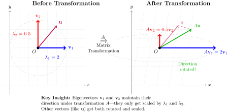
described in detail following the image
Shows a transformation that stretches and rotates, with eigenvectors as the special directions that only get scaled but not rotated.
Figure 7.1.4. Eigenvectors as Invariant Directions: How a Matrix Transforms Space
Why are eigenvectors so special? As the figure above shows, when a matrix \(A\) transforms space, most vectors get both scaled and rotated. But eigenvectors are the rare directions that only get scaled—their direction remains unchanged. This makes them the "coordinate system" in which \(A\) acts most simply. Finding these special directions is the key to understanding any linear transformation!
How do we find eigenvalues and eigenvectors? Let’s develop the method step by step.
To solve \(A\mathbf{x} = \lambda\mathbf{x}\text{,}\) we first rewrite it in standard form. Notice that:
\begin{equation*} \lambda\mathbf{x} = \lambda I_n \mathbf{x} \end{equation*}
where \(I_n\) is the \(n \times n\) identity matrix. Therefore:
\begin{align*} A\mathbf{x} \amp= \lambda\mathbf{x}\\ A\mathbf{x} \amp= \lambda I_n\mathbf{x}\\ A\mathbf{x} - \lambda I_n\mathbf{x} \amp= \mathbf{0}\\ (A - \lambda I_n)\mathbf{x} \amp= \mathbf{0} \end{align*}
This is a homogeneous system! We’ve seen these before in Chapters 2 and 4. For the system \((A - \lambda I_n)\mathbf{x} = \mathbf{0}\) to have nontrivial solutions (meaning \(\mathbf{x} \neq \mathbf{0}\)), we need the matrix \(A - \lambda I_n\) to be singular—that is, not invertible. When is a matrix singular? From Chapter 3, we know: a matrix is singular if and only if its determinant is zero.

Method for Finding Eigenvalues and Eigenvectors.

To find the eigenvalues and eigenvectors of an \(n \times n\) matrix \(A\text{:}\)
  1. Find eigenvalues: Solve the equation
    \begin{equation*} \det(A - \lambda I_n) = 0 \end{equation*}
    This gives all eigenvalues \(\lambda\text{.}\)
  2. Find eigenvectors: For each eigenvalue \(\lambda\text{,}\) solve the system
    \begin{equation*} (A - \lambda I_n)\mathbf{x} = \mathbf{0} \end{equation*}
    The nonzero solutions are the eigenvectors corresponding to \(\lambda\text{.}\)

Example 7.1.5. Finding Eigenvalues and Eigenvectors.

Find the eigenvalues and eigenvectors of the matrix
\begin{equation*} A = \begin{bmatrix} 2 \amp -12 \\ 1 \amp -5 \end{bmatrix} \end{equation*}
Solution.
Step 1: Find eigenvalues. We solve \(\det(A - \lambda I) = 0\text{:}\)
\begin{align*} \det(A - \lambda I) \amp= \det\begin{bmatrix} 2-\lambda \amp -12 \\ 1 \amp -5-\lambda \end{bmatrix}\\ \amp= (2-\lambda)(-5-\lambda) - (-12)(1)\\ \amp= -10 - 2\lambda + 5\lambda + \lambda^2 + 12\\ \amp= \lambda^2 + 3\lambda + 2\\ \amp= (\lambda + 1)(\lambda + 2) \end{align*}
Setting this equal to zero: \((\lambda + 1)(\lambda + 2) = 0\text{,}\) so \(\lambda = -1\) or \(\lambda = -2\text{.}\)
Step 2: Find eigenvectors for \(\lambda = -1\text{.}\) We solve \((A - (-1)I)\mathbf{x} = \mathbf{0}\) by finding the RREF of the augmented matrix:
\begin{equation*} \left[\begin{array}{cc|c} 3 \amp -12 \amp 0 \\ 1 \amp -4 \amp 0 \end{array}\right] \xrightarrow{\operatorname{RREF}} \left[\begin{array}{cc|c} 1 \amp -4 \amp 0 \\ 0 \amp 0 \amp 0 \end{array}\right] \end{equation*}
From the RREF, we have \(x_1 - 4x_2 = 0\text{,}\) so \(x_1 = 4x_2\text{.}\) With \(x_2 = t\) as a free variable:
\begin{equation*} \mathbf{x} = \begin{bmatrix} 4t \\ t \end{bmatrix} = t\begin{bmatrix} 4 \\ 1 \end{bmatrix} \end{equation*}
So the eigenvectors for \(\lambda = -1\) are all nonzero multiples of \(\begin{bmatrix} 4 \\ 1 \end{bmatrix}\text{.}\)
Step 3: Find eigenvectors for \(\lambda = -2\text{.}\) Similarly, solve \((A - (-2)I)\mathbf{x} = \mathbf{0}\) using RREF:
\begin{equation*} \left[\begin{array}{cc|c} 4 \amp -12 \amp 0 \\ 1 \amp -3 \amp 0 \end{array}\right] \xrightarrow{\operatorname{RREF}} \left[\begin{array}{cc|c} 1 \amp -3 \amp 0 \\ 0 \amp 0 \amp 0 \end{array}\right] \end{equation*}
From the RREF, we have \(x_1 - 3x_2 = 0\text{,}\) so \(x_1 = 3x_2\text{.}\) With \(x_2 = t\) as a free variable:
\begin{equation*} \mathbf{x} = t\begin{bmatrix} 3 \\ 1 \end{bmatrix} \end{equation*}
So the eigenvectors for \(\lambda = -2\) are all nonzero multiples of \(\begin{bmatrix} 3 \\ 1 \end{bmatrix}\text{.}\)
Let’s verify our answer using Sage:

Example 7.1.6. Finding Eigenvalues and Eigenvectors of a \(3 \times 3\) Matrix.

Find the eigenvalues and corresponding eigenvectors of the matrix
\begin{equation*} A = \begin{bmatrix} 1 \amp -1 \amp 0 \\ -1 \amp 2 \amp -1 \\ 0 \amp -1 \amp 1 \end{bmatrix} \end{equation*}
Solution.
Step 1: Find the characteristic polynomial.
We compute \(\det(A - \lambda I)\text{:}\)
\begin{align*} \det(A - \lambda I) \amp= \begin{vmatrix} 1-\lambda \amp -1 \amp 0 \\ -1 \amp 2-\lambda \amp -1 \\ 0 \amp -1 \amp 1-\lambda \end{vmatrix} \end{align*}
We can expand along the first row, but notice that the first column has a zero. Let’s do a clever row operation first: add \((1-\lambda)\) times row 2 to row 1:
\begin{align*} \amp= \begin{vmatrix} 0 \amp -1+(1-\lambda)(2-\lambda) \amp -(1-\lambda) \\ -1 \amp 2-\lambda \amp -1 \\ 0 \amp -1 \amp 1-\lambda \end{vmatrix}\\ \amp= \begin{vmatrix} 0 \amp \lambda^2-3\lambda+1 \amp \lambda-1 \\ -1 \amp 2-\lambda \amp -1 \\ 0 \amp -1 \amp 1-\lambda \end{vmatrix} \end{align*}
Now expand along the first column (only the middle entry is nonzero):
\begin{align*} \amp= (-1)^{2+1}(-1)\begin{vmatrix} \lambda^2-3\lambda+1 \amp \lambda-1 \\ -1 \amp 1-\lambda \end{vmatrix}\\ \amp= (\lambda-1)\begin{vmatrix} \lambda^2-3\lambda+1 \amp 1 \\ -1 \amp -1 \end{vmatrix}\\ \amp= (\lambda-1)[-(\ \lambda^2-3\lambda+1)+1]\\ \amp= (\lambda-1)(-\lambda^2+3\lambda)\\ \amp= -\lambda(\lambda-1)(\lambda-3) \end{align*}
The characteristic polynomial is \(p(\lambda) = -\lambda(\lambda-1)(\lambda-3)\text{,}\) so the eigenvalues are \(\lambda_1 = 0\text{,}\) \(\lambda_2 = 1\text{,}\) and \(\lambda_3 = 3\text{.}\)
Step 2: Find eigenvectors for each eigenvalue.
For \(\lambda_1 = 0\text{:}\) We solve \((A - 0I)\mathbf{x} = \mathbf{0}\text{,}\) or simply \(A\mathbf{x} = \mathbf{0}\text{.}\) Row reducing the augmented matrix:
\begin{equation*} \left[\begin{array}{rrr|r} 1 \amp -1 \amp 0 \amp 0 \\ -1 \amp 2 \amp -1 \amp 0 \\ 0 \amp -1 \amp 1 \amp 0 \end{array}\right] \xrightarrow{\operatorname{RREF}} \left[\begin{array}{rrr|r} 1 \amp 0 \amp -1 \amp 0 \\ 0 \amp 1 \amp -1 \amp 0 \\ 0 \amp 0 \amp 0 \amp 0 \end{array}\right] \end{equation*}
From the RREF, we have \(x_1 = x_3\) and \(x_2 = x_3\text{.}\) With \(x_3 = t\) as a free variable:
\begin{equation*} \mathbf{x} = t\begin{bmatrix} 1 \\ 1 \\ 1 \end{bmatrix} \end{equation*}
An eigenvector for \(\lambda_1 = 0\) is \(\mathbf{x}_1 = \begin{bmatrix} 1 \\ 1 \\ 1 \end{bmatrix}\text{.}\)
For \(\lambda_2 = 1\text{:}\) We solve \((A - I)\mathbf{x} = \mathbf{0}\text{.}\) Row reducing:
\begin{equation*} \left[\begin{array}{rrr|r} 0 \amp -1 \amp 0 \amp 0 \\ -1 \amp 1 \amp -1 \amp 0 \\ 0 \amp -1 \amp 0 \amp 0 \end{array}\right] \xrightarrow{\operatorname{RREF}} \left[\begin{array}{rrr|r} 1 \amp 0 \amp 1 \amp 0 \\ 0 \amp 1 \amp 0 \amp 0 \\ 0 \amp 0 \amp 0 \amp 0 \end{array}\right] \end{equation*}
From the RREF, we have \(x_1 = -x_3\) and \(x_2 = 0\text{.}\) With \(x_3 = t\) as a free variable:
\begin{equation*} \mathbf{x} = t\begin{bmatrix} -1 \\ 0 \\ 1 \end{bmatrix} \end{equation*}
An eigenvector for \(\lambda_2 = 1\) is \(\mathbf{x}_2 = \begin{bmatrix} -1 \\ 0 \\ 1 \end{bmatrix}\text{.}\)
For \(\lambda_3 = 3\text{:}\) We solve \((A - 3I)\mathbf{x} = \mathbf{0}\text{.}\) Row reducing:
\begin{equation*} \left[\begin{array}{rrr|r} -2 \amp -1 \amp 0 \amp 0 \\ -1 \amp -1 \amp -1 \amp 0 \\ 0 \amp -1 \amp -2 \amp 0 \end{array}\right] \xrightarrow{\operatorname{RREF}} \left[\begin{array}{rrr|r} 1 \amp 0 \amp -1 \amp 0 \\ 0 \amp 1 \amp 2 \amp 0 \\ 0 \amp 0 \amp 0 \amp 0 \end{array}\right] \end{equation*}
From the RREF, we have \(x_1 = x_3\) and \(x_2 = -2x_3\text{.}\) With \(x_3 = t\) as a free variable:
\begin{equation*} \mathbf{x} = t\begin{bmatrix} 1 \\ -2 \\ 1 \end{bmatrix} \end{equation*}
An eigenvector for \(\lambda_3 = 3\) is \(\mathbf{x}_3 = \begin{bmatrix} 1 \\ -2 \\ 1 \end{bmatrix}\text{.}\)
Summary: The eigenvalues and corresponding eigenvectors are:
  • \(\lambda_1 = 0\text{:}\) eigenvector \(\begin{bmatrix} 1 \\ 1 \\ 1 \end{bmatrix}\)
  • \(\lambda_2 = 1\text{:}\) eigenvector \(\begin{bmatrix} -1 \\ 0 \\ 1 \end{bmatrix}\)
  • \(\lambda_3 = 3\text{:}\) eigenvector \(\begin{bmatrix} 1 \\ -2 \\ 1 \end{bmatrix}\)
Checkpoint 7.1.7. Finding Eigenvalues and Eigenvectors of a \(3 \times 3\) Matrix.

Find the eigenvalues and eigenvectors of the matrix
\begin{equation*} B = \begin{bmatrix} 1 \amp 2 \amp -2 \\ -2 \amp 5 \amp -2 \\ -6 \amp 6 \amp -3 \end{bmatrix} \end{equation*}
Hint.
Compute the characteristic polynomial \(p(\lambda) = \det(B - \lambda I)\) by expanding the \(3 \times 3\) determinant along the first row. After simplifying, you will obtain a cubic polynomial \(-\lambda^3 + 3\lambda^2 + 9\lambda - 27\text{.}\) Try factoring by grouping: write \(\lambda^2(\lambda - 3) - 9(\lambda - 3) = 0\) and identify the common factor.
Solution.
Step 1: Find the eigenvalues.
We compute \(\det(B - \lambda I) = 0\text{:}\)
\begin{equation*} B - \lambda I = \begin{bmatrix} 1-\lambda \amp 2 \amp -2 \\ -2 \amp 5-\lambda \amp -2 \\ -6 \amp 6 \amp -3-\lambda \end{bmatrix} \end{equation*}
Expanding along the first row, it is not hard to see that
\begin{equation*} \det(B - \lambda I)=-\lambda^3 + 3\lambda^2 + 9\lambda - 27 \end{equation*}
It is a chanllenge to factor this cubic polynomial. We try to "guess" a root by testing small integer factors of 27. We find that \(\lambda = 3\) is a root, so we can factor out \(\lambda - 3\text{:}\)
\begin{equation*} -\lambda^3 + 3\lambda^2 + 9\lambda - 27 = -(\lambda - 3)(\lambda^2 + a\lambda + b). \end{equation*}
A simple computation yileds that \(a=0\) and \(b=-9\text{,}\) so
\begin{equation*} -\lambda^3 + 3\lambda^2 + 9\lambda - 27 = -(\lambda - 3)(\lambda^2 - 9) = -(\lambda - 3)^2(\lambda + 3) \end{equation*}
The eigenvalues are \(\lambda_1 = 3\)and \(\lambda_2 = -3\text{.}\)
Step 2: Find the eigenvectors for \(\lambda_1 = 3\text{.}\)
We solve \((B - 3I)\mathbf{x} = \mathbf{0}\text{.}\) The augmented matrix row reduces as follows:
\begin{equation*} \left[\begin{array}{ccc|c} -2 \amp 2 \amp -2 \amp 0 \\ -2 \amp 2 \amp -2 \amp 0 \\ -6 \amp 6 \amp -6 \amp 0 \end{array}\right] \xrightarrow{\operatorname{RREF}} \left[\begin{array}{ccc|c} 1 \amp -1 \amp 1 \amp 0 \\ 0 \amp 0 \amp 0 \amp 0 \\ 0 \amp 0 \amp 0 \amp 0 \end{array}\right] \end{equation*}
From the RREF, \(x_1 = x_2 - x_3\text{,}\) with \(x_2 = s\) and \(x_3 = t\) free:
\begin{equation*} \mathbf{x} = s\begin{bmatrix}1\\1\\0\end{bmatrix} + t\begin{bmatrix}-1\\0\\1\end{bmatrix}, \quad (s, t) \neq (0,0) \end{equation*}
which is an eigenvector for \(\lambda_1 = 3\text{.}\)
Step 3: Find the eigenvectors for \(\lambda_2 = -3\text{.}\)
We solve \((B + 3I)\mathbf{x} = \mathbf{0}\text{.}\) The augmented matrix row reduces as follows:
\begin{equation*} \left[\begin{array}{ccc|c} 4 \amp 2 \amp -2 \amp 0 \\ -2 \amp 8 \amp -2 \amp 0 \\ -6 \amp 6 \amp 0 \amp 0 \end{array}\right] \xrightarrow{\operatorname{RREF}} \left[\begin{array}{ccc|c} 1 \amp 0 \amp -\frac{1}{3} \amp 0 \\ 0 \amp 1 \amp -\frac{1}{3} \amp 0 \\ 0 \amp 0 \amp 0 \amp 0 \end{array}\right] \end{equation*}
From the RREF, \(x_1 = \frac{1}{3}x_3\) and \(x_2 = \frac{1}{3}x_3\text{.}\) Setting \(x_3 = 3t\text{:}\)
\begin{equation*} \mathbf{x} = t\begin{bmatrix}1\\1\\3\end{bmatrix}, \quad t \neq 0 \end{equation*}
which is an eigenvector for \(\lambda_2 = -3\text{.}\)

Remark 7.1.8.

A matrix may have no eigenvalues at all! For example, the matrix \(\begin{bmatrix} 0 \amp -1 \\ 1 \amp 0 \end{bmatrix}\) has characteristic polynomial \(\lambda^2 + 1\text{,}\) which has no real roots. However, if we allow complex numbers, then every matrix has eigenvalues.

Subsection 7.1.2 The Characteristic Polynomial

The equation \(\det(A - \lambda I_n) = 0\) that we solve to find eigenvalues is actually a polynomial equation in \(\lambda\text{.}\) This polynomial deserves a name.

Definition 7.1.9. Characteristic Polynomial.

Let \(A\) be an \(n \times n\) matrix. The polynomial
\begin{equation*} p(\lambda) = \det(A-\lambda I_n) \end{equation*}
is called the characteristic polynomial of \(A\text{.}\)
The eigenvalues of \(A\) are precisely the roots of the characteristic polynomial.

Remark 7.1.10. Sign Convention.

Some textbooks define the characteristic polynomial as \(\det( \lambda I-A)\) instead of \(\det(A - \lambda I)\text{.}\) These differ only by a factor of \((-1)^n\text{,}\) so they have the same roots (eigenvalues). In this book, we use \(\det(A - \lambda I)\) to avoid changing the signs of numbers in \(A\text{.}\)

Insight 7.1.11. Properties of the Characteristic Polynomial.

For an \(n \times n\) matrix \(A\text{,}\) the characteristic polynomial \(p(\lambda) = \det(A - \lambda I)\) is a polynomial of degree \(n\text{.}\) By the Fundamental Theorem of Algebra (allowing complex numbers), it has exactly \(n\) roots (counting multiplicities).
This means: every \(n \times n\) matrix has exactly \(n\) eigenvalues (counting multiplicities), though some may be complex numbers.
Let’s practice computing characteristic polynomials using Sage:

Example 7.1.12. Computing Characteristic Polynomials.

Find the characteristic polynomial of the matrices \(A\) and \(B\) from the previous examples.

Proof.

The matrix \(\lambda I - A\) is also upper triangular, with diagonal entries \((\lambda - a_{11}), (\lambda - a_{22}), \ldots, (\lambda - a_{nn})\text{.}\) The determinant of a triangular matrix is the product of its diagonal entries, so:
\begin{equation*} \det(\lambda I - A) = (\lambda - a_{11})(\lambda - a_{22})\cdots(\lambda - a_{nn}) \end{equation*}
The roots of this polynomial are exactly \(a_{11}, a_{22}, \ldots, a_{nn}\text{.}\)

Example 7.1.14.

Find the eigenvalues of
\begin{equation*} A = \begin{bmatrix} 1 \amp -2 \amp 1 \\ 0 \amp 0 \amp 1 \\ 0 \amp 0 \amp -3 \end{bmatrix} \end{equation*}
Solution.
Since \(A\) is upper triangular, the eigenvalues are simply the diagonal entries: \(\lambda = 1, 0, -3\text{.}\)

Proof.

We need to show that \(\det(\lambda I - A) = \det(\lambda I - B)\text{.}\) Starting with the definition of \(B\text{:}\)
\begin{align*} \det(\lambda I - B) \amp = \det(\lambda I - P^{-1}AP)\\ \amp = \det(P^{-1}(\lambda I)P - P^{-1}AP) \amp \amp \text{(since } P^{-1}(\lambda I)P = \lambda P^{-1}IP = \lambda I\text{)}\\ \amp = \det(P^{-1}(\lambda I - A)P)\\ \amp = \det(P^{-1}) \cdot \det(\lambda I - A) \cdot \det(P) \amp \amp \text{(multiplicative property)}\\ \amp = \det(P^{-1}) \cdot \det(P) \cdot \det(\lambda I - A)\\ \amp = \det(P^{-1}P) \cdot \det(\lambda I - A) \amp \amp \text{(multiplicative property)}\\ \amp = \det(I) \cdot \det(\lambda I - A)\\ \amp = 1 \cdot \det(\lambda I - A)\\ \amp = \det(\lambda I - A) \end{align*}
Therefore, \(A\) and \(B\) have the same characteristic polynomial, and hence the same eigenvalues with the same algebraic multiplicities.

Remark 7.1.16. Why This Matters.

This theorem tells us that similarity is an equivalence relation that preserves eigenvalues. Two matrices that represent the same linear transformation in different bases (hence similar) must have the same eigenvalues—a fundamental invariant of the transformation itself, independent of the choice of basis.
Warning: The converse is not true. Two matrices can have the same eigenvalues without being similar. For example, \(I = \begin{bmatrix} 1 \amp 0 \\ 0 \amp 1 \end{bmatrix}\) and \(A = \begin{bmatrix} 1 \amp 1 \\ 0 \amp 1 \end{bmatrix}\) both have eigenvalue \(\lambda = 1\) (with multiplicity 2), but they are not similar because \(I\) is diagonalizable while \(A\) is not.

Subsection 7.1.3 Eigenspaces

For each eigenvalue of a matrix, there is an entire collection of eigenvectors. This collection, together with the zero vector, forms an important structure.

Definition 7.1.17. Eigenspace.

Let \(A\) be an \(n \times n\) matrix and \(\lambda\) an eigenvalue of \(A\text{.}\) The eigenspace of \(A\) corresponding to \(\lambda\text{,}\) denoted \(E_\lambda\text{,}\) is the set of all eigenvectors corresponding to \(\lambda\text{,}\) together with the zero vector:
\begin{equation*} E_\lambda = \{\mathbf{x} \in \mathbb{R}^n : A\mathbf{x} = \lambda\mathbf{x}\} = \{\mathbf{x} \in \mathbb{R}^n : (A - \lambda I)\mathbf{x} = \mathbf{0}\} \end{equation*}
In other words, \(E_\lambda = \operatorname{Nul}(A - \lambda I)\text{,}\) the null space (kernel) of the matrix \(A - \lambda I\text{.}\)
Notice that the eigenspace consists of:
  • All eigenvectors corresponding to \(\lambda\)
  • The zero vector \(\mathbf{0}\)
We include \(\mathbf{0}\) even though it is not an eigenvector, because this makes \(E_\lambda\) a subspace, as we now prove.

Proof.

Since \(E_\lambda = \operatorname{Nul}(A - \lambda I)\text{,}\) and the null space of any matrix is a subspace, it follows that \(E_\lambda\) is a subspace of \(\mathbb{R}^n\text{.}\)
Alternatively, we can verify the subspace axioms directly:
(1) Zero vector: \((A - \lambda I)\mathbf{0} = \mathbf{0}\text{,}\) so \(\mathbf{0} \in E_\lambda\text{.}\)
(2) Closure under addition: If \(\mathbf{u}, \mathbf{v} \in E_\lambda\text{,}\) then \(A\mathbf{u} = \lambda\mathbf{u}\) and \(A\mathbf{v} = \lambda\mathbf{v}\text{.}\) Therefore:
\begin{equation*} A(\mathbf{u} + \mathbf{v}) = A\mathbf{u} + A\mathbf{v} = \lambda\mathbf{u} + \lambda\mathbf{v} = \lambda(\mathbf{u} + \mathbf{v}) \end{equation*}
So \(\mathbf{u} + \mathbf{v} \in E_\lambda\text{.}\)
(3) Closure under scalar multiplication: If \(\mathbf{u} \in E_\lambda\) and \(c \in \mathbb{R}\text{,}\) then \(A\mathbf{u} = \lambda\mathbf{u}\text{.}\) Therefore:
\begin{equation*} A(c\mathbf{u}) = c(A\mathbf{u}) = c(\lambda\mathbf{u}) = \lambda(c\mathbf{u}) \end{equation*}
So \(c\mathbf{u} \in E_\lambda\text{.}\)
Since all three subspace axioms hold, \(E_\lambda\) is a subspace of \(\mathbb{R}^n\text{.}\)
This theorem has important consequences:
  • The eigenspace \(E_\lambda=\operatorname{Nullspace}(A-\lambda I)\text{.}\)
  • Any linear combination of eigenvectors for \(\lambda\) is also an eigenvector for \(\lambda\) (or the zero vector).
  • The eigenspace \(E_\lambda\) has a basis and a dimension.
  • To find all eigenvectors for \(\lambda\text{,}\) we need only find a basis for \(E_\lambda\text{.}\)

Example 7.1.19. Finding a Basis for an Eigenspace.

For the matrix \(A = \begin{bmatrix} 2 \amp -12 \\ 1 \amp -5 \end{bmatrix}\text{,}\) we found in Example 7.1.5 that \(\lambda = -1\) is an eigenvalue. Find a basis for the eigenspace \(E_{-1}\) and determine its dimension.
Solution.
We solve \((A - (-1)I)\mathbf{x} = \mathbf{0}\) by finding the RREF of the augmented matrix:
\begin{equation*} \left[\begin{array}{cc|c} 3 \amp -12 \amp 0 \\ 1 \amp -4 \amp 0 \end{array}\right] \xrightarrow{\operatorname{RREF}} \left[\begin{array}{cc|c} 1 \amp -4 \amp 0 \\ 0 \amp 0 \amp 0 \end{array}\right] \end{equation*}
From the RREF, we have \(x_1 - 4x_2 = 0\text{,}\) so \(x_1 = 4x_2\text{.}\) With \(x_2 = t\) as a free variable:
\begin{equation*} \mathbf{x} = \begin{bmatrix} 4t \\ t \end{bmatrix} = t\begin{bmatrix} 4 \\ 1 \end{bmatrix} \end{equation*}
Therefore, the eigenspace \(E_{-1}\) is:
\begin{equation*} E_{-1} = \operatorname{span}\left\{\begin{bmatrix} 4 \\ 1 \end{bmatrix}\right\} \end{equation*}
A basis for \(E_{-1}\) is \(\left\{\begin{bmatrix} 4 \\ 1 \end{bmatrix}\right\}\text{,}\) and \(\dim(E_{-1}) = 1\text{.}\)
Geometric interpretation: The eigenspace \(E_{-1}\) is a one-dimensional subspace (a line through the origin) in \(\mathbb{R}^2\text{.}\) Every vector on this line is either an eigenvector for \(\lambda = -1\) or the zero vector.

Checkpoint 7.1.20. Finding Eigenspaces of a \(3 \times 3\) Matrix.

Consider the matrix
\begin{equation*} B = \begin{bmatrix} 1 \amp 2 \amp -2 \\ -2 \amp 5 \amp -2 \\ -6 \amp 6 \amp -3 \end{bmatrix} \end{equation*}
  1. Find a basis for each eigenspace \(E_{\lambda}\) for each eigenvalue \(\lambda\) of \(B\text{.}\)
  2. What is the dimension of each eigenspace?
Hint.
From Checkpoint 7.1.7, we found that the eigenvalues are \(\lambda_1 = 3\) (with algebraic multiplicity 2) and \(\lambda_2 = -3\) (with algebraic multiplicity 1). For each eigenvalue, the eigenspace is \(E_{\lambda} = \operatorname{Nul}(B - \lambda I)\text{.}\)
Solution.
From Checkpoint 7.1.7, we have:
Eigenspace \(E_3\) for \(\lambda_1 = 3\text{:}\)
We found that \((B - 3I)\mathbf{x} = \mathbf{0}\) has general solution:
\begin{equation*} \mathbf{x} = s\begin{bmatrix}1\\1\\0\end{bmatrix} + t\begin{bmatrix}-1\\0\\1\end{bmatrix}, \quad s, t \in \mathbb{R} \end{equation*}
Therefore, the eigenspace is:
\begin{equation*} E_3 = \operatorname{span}\left\{\begin{bmatrix}1\\1\\0\end{bmatrix},\, \begin{bmatrix}-1\\0\\1\end{bmatrix}\right\} \end{equation*}
A basis for \(E_3\) is \(\left\{\begin{bmatrix}1\\1\\0\end{bmatrix},\, \begin{bmatrix}-1\\0\\1\end{bmatrix}\right\}\text{,}\) and \(\dim(E_3) = 2\text{.}\)
Geometric interpretation: The eigenspace \(E_3\) is a two-dimensional subspace (a plane through the origin) in \(\mathbb{R}^3\text{.}\) Every nonzero vector in this plane is an eigenvector for \(\lambda = 3\text{.}\)
Eigenspace \(E_{-3}\) for \(\lambda_2 = -3\text{:}\)
We found that \((B + 3I)\mathbf{x} = \mathbf{0}\) has general solution:
\begin{equation*} \mathbf{x} = t\begin{bmatrix}1\\1\\3\end{bmatrix}, \quad t \in \mathbb{R} \end{equation*}
Therefore, the eigenspace is:
\begin{equation*} E_{-3} = \operatorname{span}\left\{\begin{bmatrix}1\\1\\3\end{bmatrix}\right\} \end{equation*}
A basis for \(E_{-3}\) is \(\left\{\begin{bmatrix}1\\1\\3\end{bmatrix}\right\}\text{,}\) and \(\dim(E_{-3}) = 1\text{.}\)
Geometric interpretation: The eigenspace \(E_{-3}\) is a one-dimensional subspace (a line through the origin) in \(\mathbb{R}^3\text{.}\) Every nonzero vector on this line is an eigenvector for \(\lambda = -3\text{.}\)
The dimension of an eigenspace will play a crucial role in determining whether a matrix can be diagonalized, as we will see in the next subsection.

Subsection 7.1.4 Algebraic and Geometric Multiplicities

We now introduce two important concepts: algebraic and geometric multiplicity.
Suppose the characteristic polynomial of a matrix \(A\) factors as:
\begin{equation*} p(\lambda) = (\lambda - \lambda_1)^{m_1}(\lambda - \lambda_2)^{m_2}\cdots(\lambda - \lambda_k)^{m_k} \end{equation*}
where \(\lambda_1, \lambda_2, \ldots, \lambda_k\) are the distinct eigenvalues.

Definition 7.1.21. Algebraic Multiplicity.

The algebraic multiplicity of an eigenvalue \(\lambda_i\) is the exponent \(m_i\) in the factorization of the characteristic polynomial—that is, the number of times \(\lambda_i\) appears as a root (counting repetitions).
However, just because \(\lambda\) is a repeated root doesn’t mean we automatically get multiple linearly independent eigenvectors! The number of linearly independent eigenvectors is measured by the geometric multiplicity.

Definition 7.1.22. Geometric Multiplicity.

The geometric multiplicity of an eigenvalue \(\lambda\) is the dimension of the eigenspace.
Equivalently, it equals \(\text{nullity}(A - \lambda I)\text{,}\) the dimension of the null space of \(A - \lambda I\text{.}\)

Insight 7.1.23. Key Relationship.

For any eigenvalue \(\lambda\text{,}\) we always have:
\begin{equation*} 1 \leq \text{geometric multiplicity} \leq \text{algebraic multiplicity} \end{equation*}
  • The geometric multiplicity is at least 1 because there must be at least one eigenvector (by definition of eigenvalue).
  • The geometric multiplicity cannot exceed the algebraic multiplicity (Hint: Use the Theorem 7.1.15).
Why this matters: A matrix is diagonalizable if and only if, for every eigenvalue, geometric multiplicity equals algebraic multiplicity. When geometric multiplicity is less than algebraic multiplicity, we don’t have enough eigenvectors to diagonalize!

Example 7.1.24. Computing Multiplicities.

Find the algebraic and geometric multiplicities of all eigenvalues of
\begin{equation*} A = \begin{bmatrix} 2 \amp 1 \amp 0 \\ 0 \amp 2 \amp 0 \\ 0 \amp 0 \amp 2 \end{bmatrix} \end{equation*}
Solution.
Step 1: Find the characteristic polynomial.
\begin{equation*} \det(\lambda I - A) = \det\begin{bmatrix} \lambda-2 \amp -1 \amp 0 \\ 0 \amp \lambda-2 \amp 0 \\ 0 \amp 0 \amp \lambda-2 \end{bmatrix} = (\lambda-2)^3 \end{equation*}
So the only eigenvalue is \(\lambda = 2\) with algebraic multiplicity \(3\text{.}\)
Step 2: Find the geometric multiplicity. We solve \((A - 2I)\mathbf{x} = \mathbf{0}\) by finding the RREF:
\begin{equation*} \left[\begin{array}{ccc|c} 0 \amp 1 \amp 0 \amp 0 \\ 0 \amp 0 \amp 0 \amp 0 \\ 0 \amp 0 \amp 0 \amp 0 \end{array}\right] \xrightarrow{\operatorname{RREF}} \left[\begin{array}{ccc|c} 0 \amp 1 \amp 0 \amp 0 \\ 0 \amp 0 \amp 0 \amp 0 \\ 0 \amp 0 \amp 0 \amp 0 \end{array}\right] \end{equation*}
From the RREF, we have \(x_2 = 0\text{,}\) while \(x_1\) and \(x_3\) are free variables. So the eigenspace has dimension \(2\) with basis \(\{\begin{bmatrix} 1 \\ 0 \\ 0 \end{bmatrix}, \begin{bmatrix} 0 \\ 0 \\ 1 \end{bmatrix}\}\text{.}\)
Conclusion: For \(\lambda = 2\text{:}\) algebraic multiplicity = 3, geometric multiplicity = 2. Since these are unequal, \(A\) is not diagonalizable!

Connecting the Concepts.

The eigenspace \(E_\lambda\) is a subspace of \(\mathbb{R}^n\) (we learned about subspaces in Chapter 4). Its dimension is the geometric multiplicity of \(\lambda\text{.}\) This connects three major concepts:
  • Eigenspaces (from eigen-theory)
  • Null spaces (from solving linear systems)
  • Subspaces and dimension (from vector space theory)
Once again, we see how different parts of linear algebra fit together!

Subsection 7.1.5 Property of Eigenvectors

In this part, we always assume that \(A\) is an \(n \times n\) matrix and \(\lambda\in \mathbb{R}\) is an eigenvalue of \(A\) with corresponding eigenvector \(v\text{.}\)

Proof.

Suppose for contradiction that \(v_1 + v_2\) is an eigenvector of \(A\) with eigenvalue \(\mu\text{.}\) Then:
\begin{equation*} A(v_1 + v_2) = \mu(v_1 + v_2) \end{equation*}
On the other hand, since \(Av_1 = \lambda_1 v_1\) and \(Av_2 = \lambda_2 v_2\text{:}\)
\begin{equation*} A(v_1 + v_2) = \lambda_1 v_1 + \lambda_2 v_2 \end{equation*}
Combining these two equations gives:
\begin{equation*} \lambda_1 v_1 + \lambda_2 v_2 = \mu v_1 + \mu v_2 \end{equation*}
which simplifies to:
\begin{equation*} (\lambda_1 - \mu)v_1 + (\lambda_2 - \mu)v_2 = \mathbf{0} \end{equation*}
By Lemma 7.1.27, \(\{v_1, v_2\}\) is linearly independent (since \(\lambda_1 \neq \lambda_2\)). Therefore \(\lambda_1 - \mu = 0\) and \(\lambda_2 - \mu = 0\text{,}\) giving \(\lambda_1 = \mu = \lambda_2\text{.}\) This contradicts the assumption that \(\lambda_1 \neq \lambda_2\text{.}\)
We have seen that eigenvectors corresponding to a given eigenvalue form a subspace (the eigenspace). What about eigenvectors corresponding to different eigenvalues? Do they have any special relationship?

Proof.

We will prove this by induction on \(k\text{.}\)
  • Base case: If \(k = 1\text{,}\) then \(\{v_1\}\) is linearly independent since \(v_1 \neq \mathbf{0}\text{.}\)
  • Inductive step: Assume the statement holds for any set of \(k-1\) eigenvectors corresponding to distinct eigenvalues.
  • Now consider a set of \(k\) eigenvectors \(\{v_1, v_2, \dots, v_k\}\) corresponding to distinct eigenvalues \(\lambda_1, \lambda_2, \dots, \lambda_k\text{.}\) Suppose
    \begin{equation*} c_1 v_1 + c_2 v_2 + \cdots + c_k v_k = \mathbf{0}\tag{1} \end{equation*}
    Applying \(A\) to both sides gives:
    \begin{equation*} c_1 \lambda_1 v_1 + c_2 \lambda_2 v_2 + \cdots + c_k \lambda_k v_k = \mathbf{0}\tag{2} \end{equation*}
    Subtracting \(\lambda_1\) times equation (1) from the equation (2) gives:
    \begin{equation*} c_2 (\lambda_2 - \lambda_1) v_2 + \cdots + c_k (\lambda_k - \lambda_1) v_k = \mathbf{0} \end{equation*}
    By the inductive hypothesis, \(\{v_2, \dots, v_k\}\) is linearly independent, so \(c_2 (\lambda_2 - \lambda_1) = 0\text{,}\) \(c_3 (\lambda_3 - \lambda_1) = 0\text{,}\) ..., \(c_k (\lambda_k - \lambda_1) = 0\text{.}\) Since the eigenvalues are distinct, \(\lambda_i - \lambda_1 \neq 0\) for all \(i \geq 2\text{,}\) so we must have \(c_2 = c_3 = \cdots = c_k = 0\text{.}\) Substituting back into the first equation gives \(c_1 v_1 = \mathbf{0}\text{,}\) so \(c_1 = 0\text{.}\) Therefore, \(c_1 = c_2 = \cdots = c_k = 0\text{,}\) and \(\{v_1, v_2, \dots, v_k\}\) is linearly independent.
By induction, the statement holds for all \(k \in \mathbb{N}\text{.}\)

